Download as PDF, PPTX

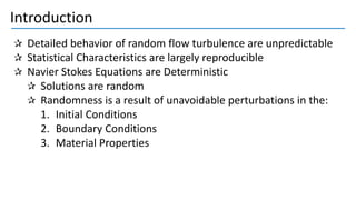
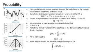
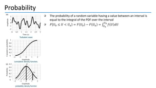
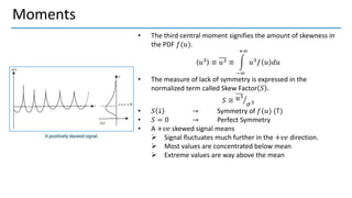
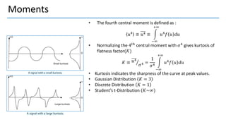
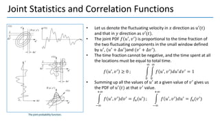
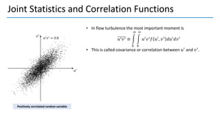

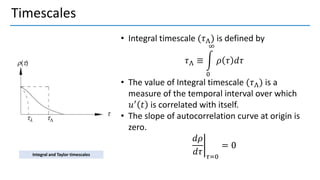
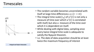
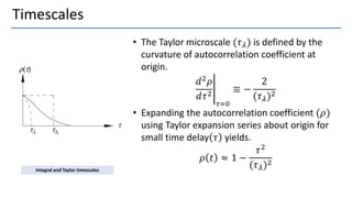
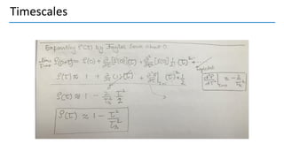
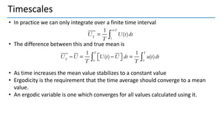

This document provides an overview of statistical descriptions and characteristics of turbulence. It discusses: 1. Turbulence is unpredictable in detail but its statistical characteristics are largely reproducible. Solutions to the Navier-Stokes equations are random due to unavoidable perturbations. 2. Probability density functions, cumulative distribution functions, moments like mean, variance, skewness, kurtosis are used to statistically characterize turbulence. 3. Autocorrelation functions describe how turbulence variables correlate over time and space; integral and Taylor time scales measure temporal correlations.