Download as PDF, PPTX


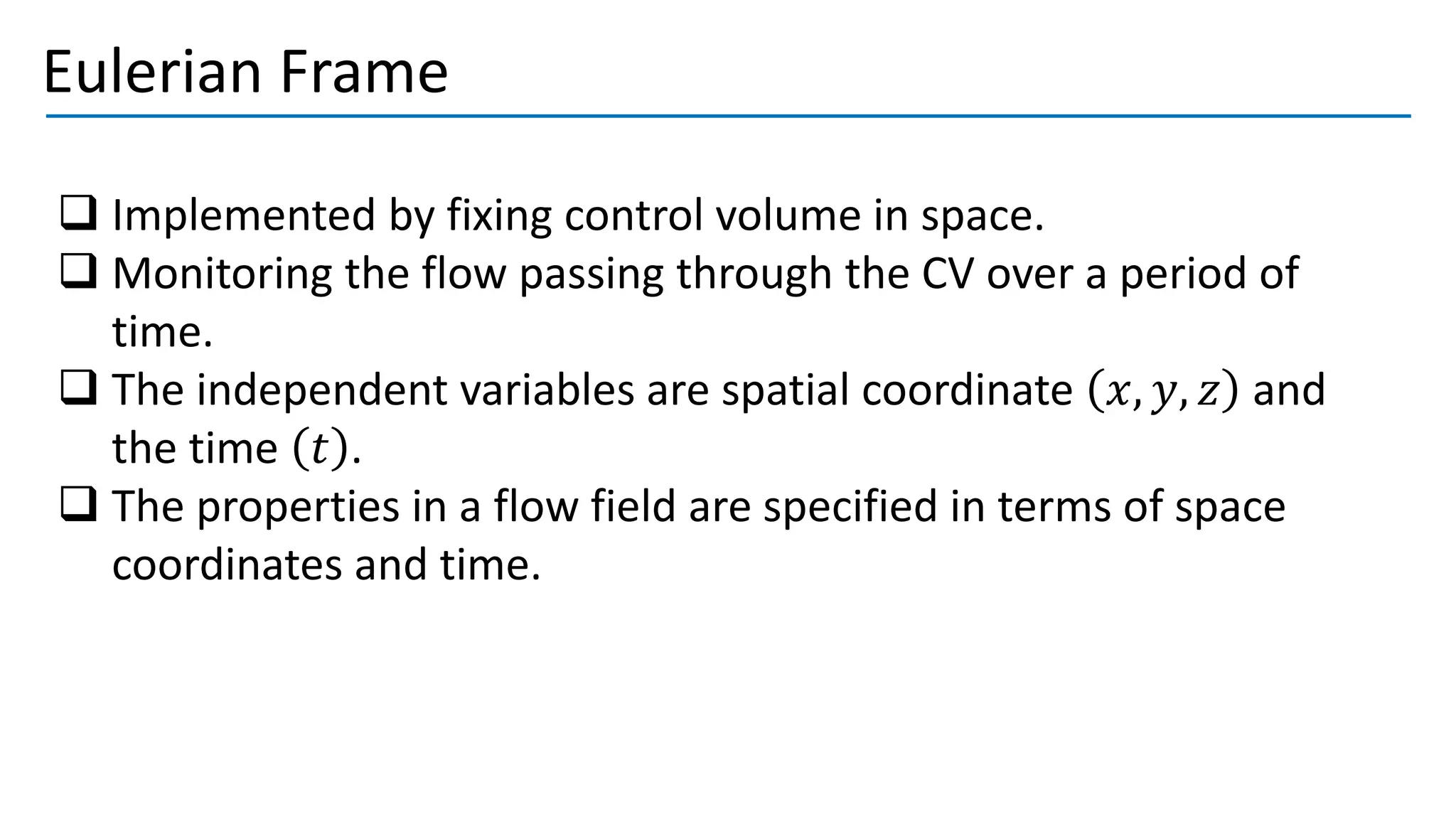
![Eulerian Frame
www.youtube.com. (n.d.). YouTube. [online] Available at:https://www.youtube.com/watch?v=IxOt4ALui8k.](https://image.slidesharecdn.com/basicsofturbulencefinal-210422003305/75/Basics-of-Turbulent-Flow-39-2048.jpg)
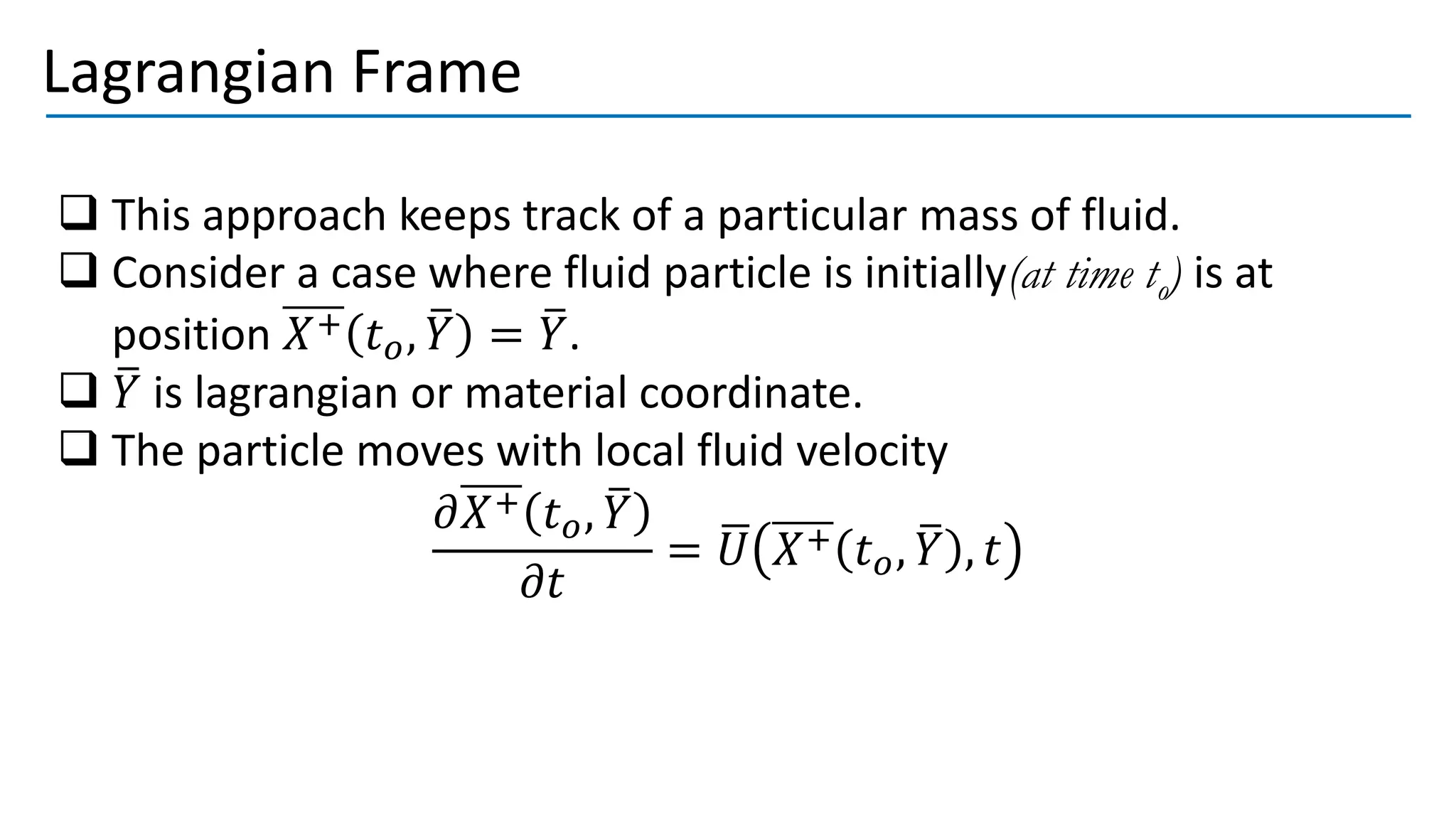
![Lagrangian Frame
www.youtube.com. (n.d.). YouTube. [online] Available at:https://www.youtube.com/watch?v=SsnYoqdFGIY&t=1s.](https://image.slidesharecdn.com/basicsofturbulencefinal-210422003305/75/Basics-of-Turbulent-Flow-40-2048.jpg)


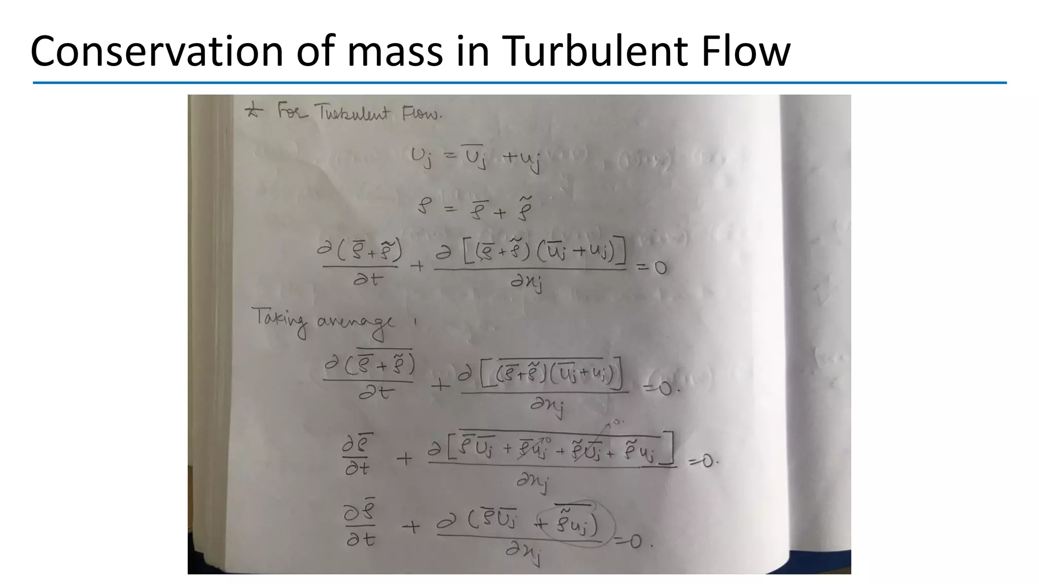

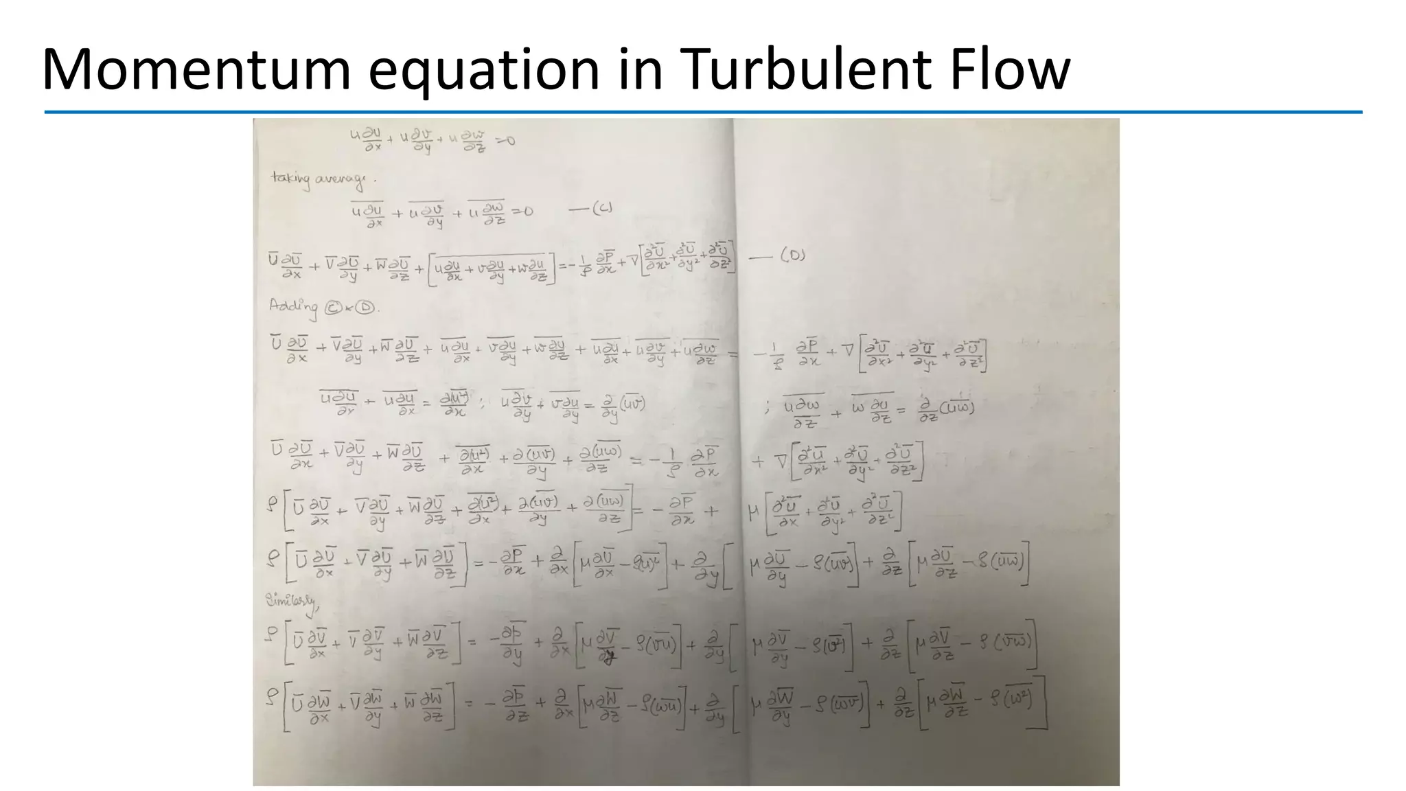
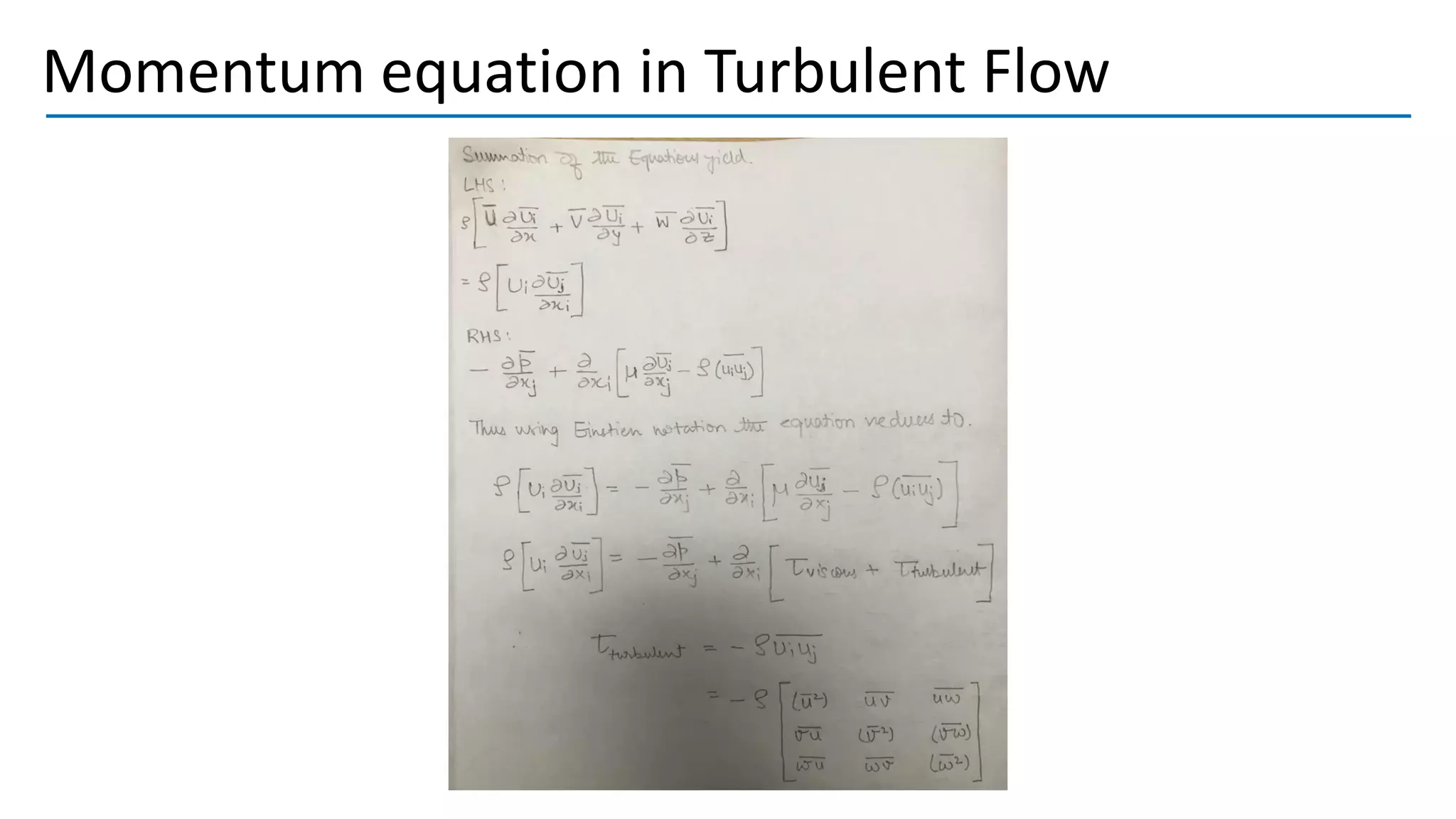
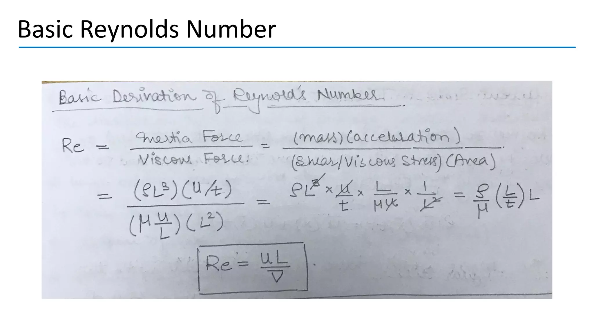
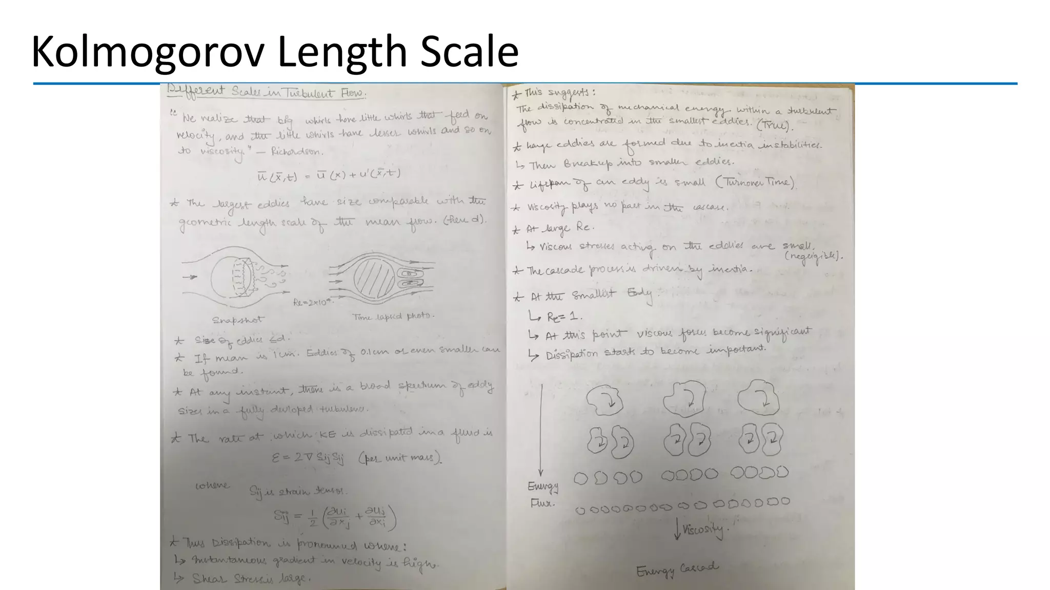


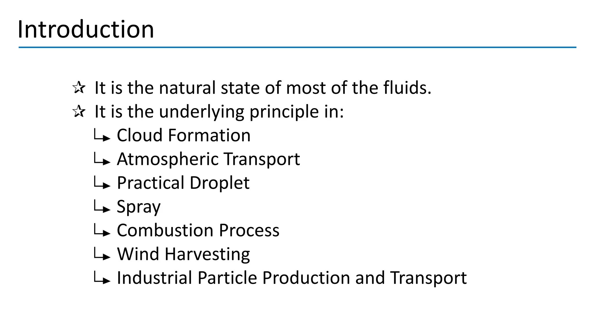
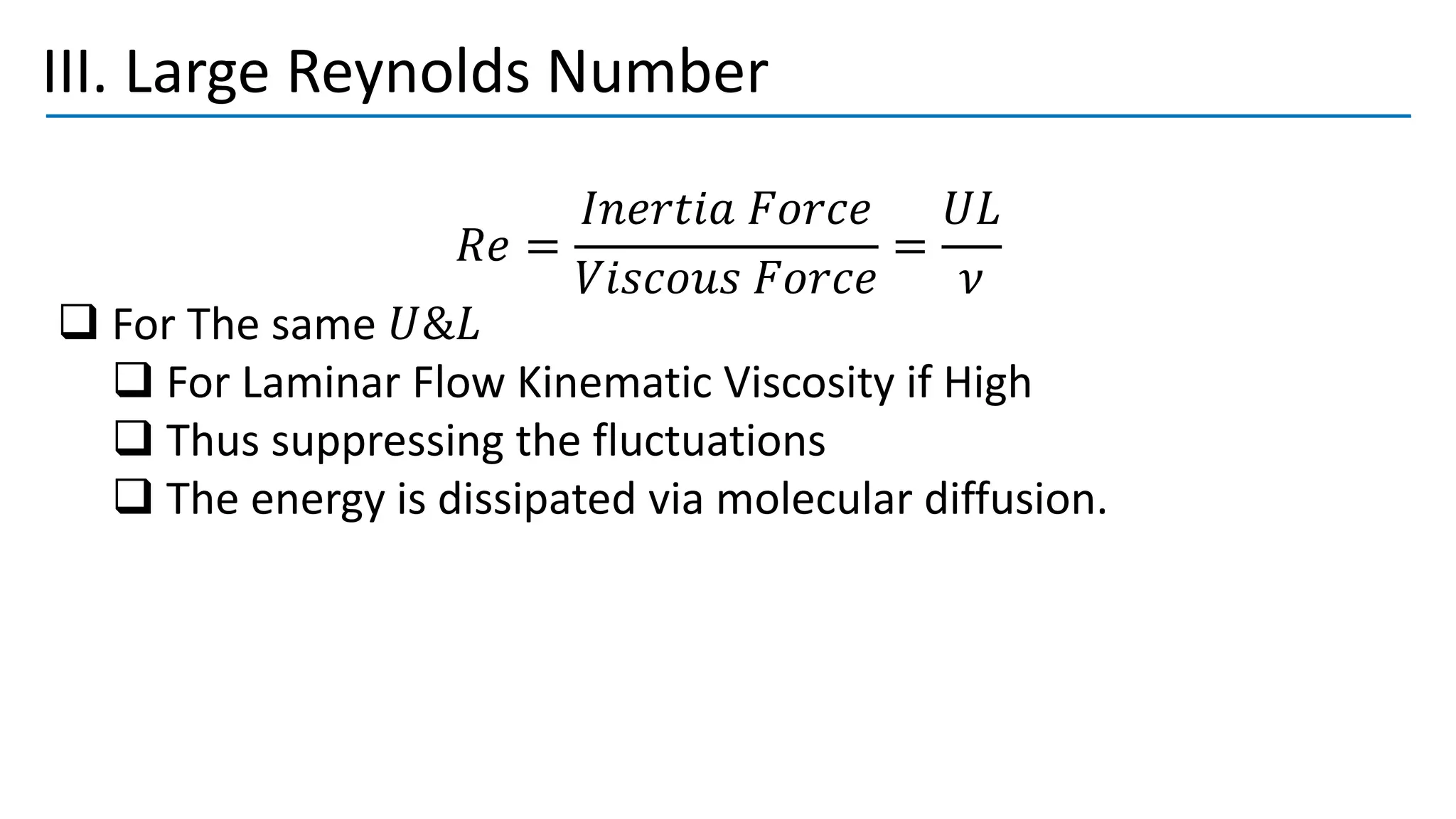
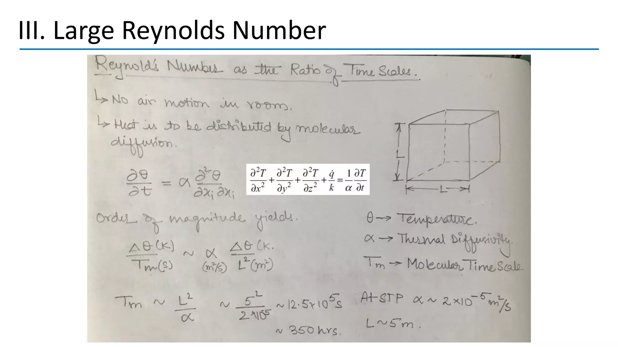
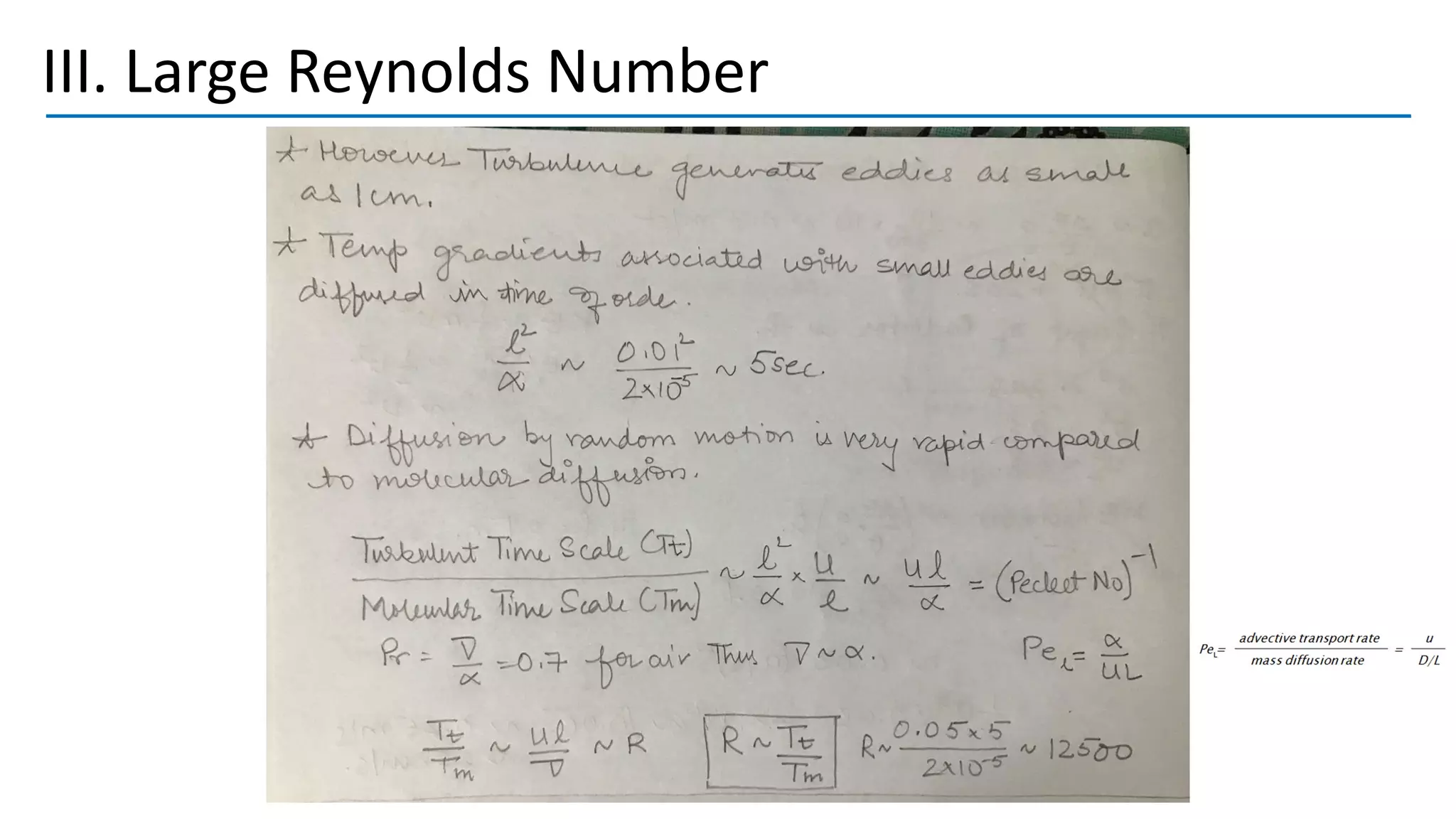
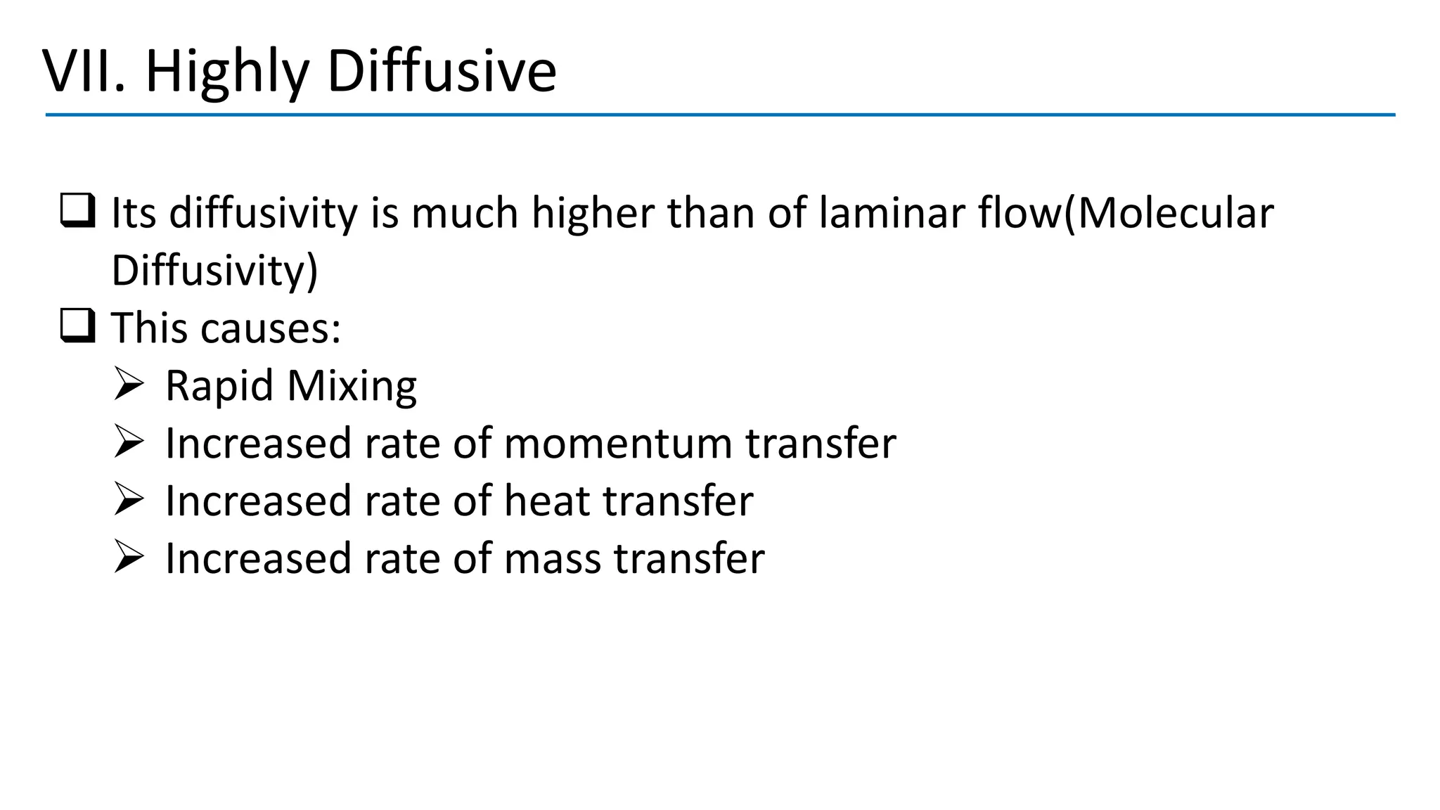
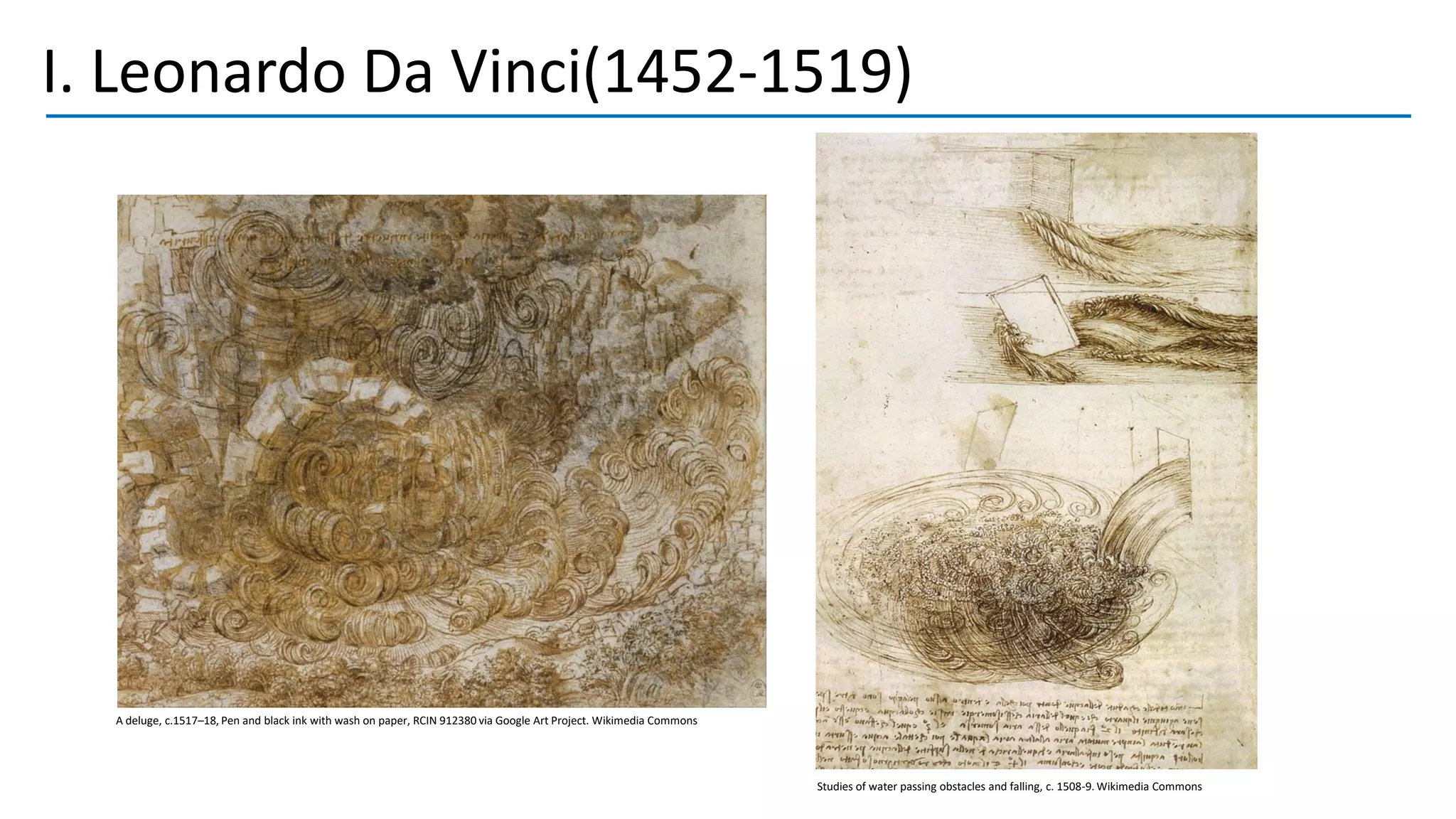
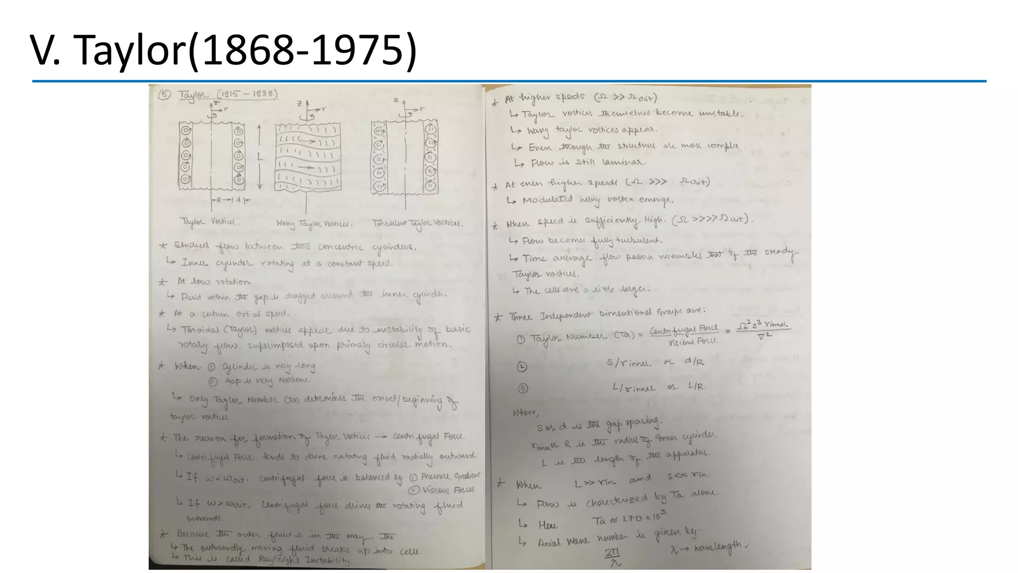
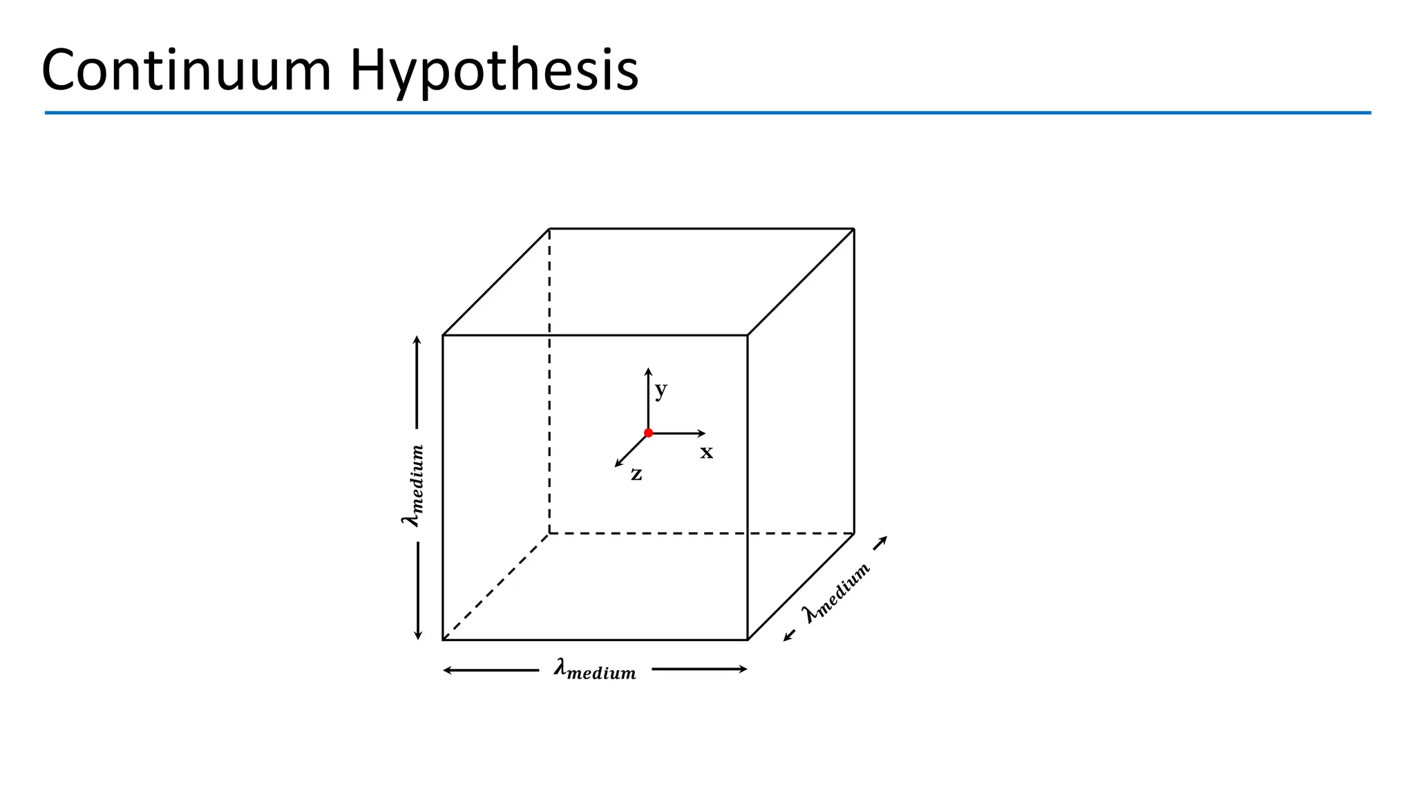
Turbulent flow is characterized by randomness, irregularity, and fluctuations across a wide range of length and time scales. It occurs at high Reynolds numbers where inertial forces dominate over viscous forces. Key features include being 3D, highly diffusive, dissipative, and containing many vortices. The equations that govern fluid motion, such as the continuity and Navier-Stokes equations, can still be applied through use of the continuum hypothesis even when modeling turbulent flow as a continuum phenomenon. Turbulence was first studied scientifically by figures such as Leonardo da Vinci, Osborne Reynolds, and Ludwig Prandtl, laying the foundations for further research.