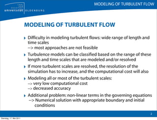
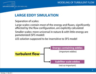
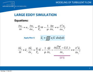
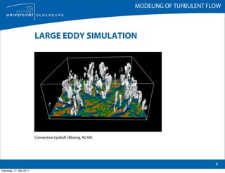
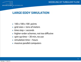
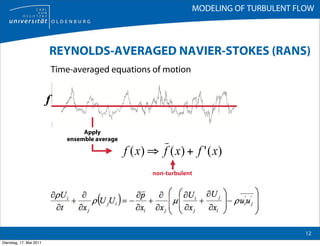
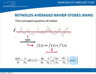
WIND ENERGY METEOROLOGY

                         UNIT 5
                         MODELING OF TURBULENT FLOW


                         Detlev Heinemann

                         ENERGY METEOROLOGY GROUP
                         INSTITUTE OF PHYSICS
                         OLDENBURG UNIVERSITY
                         FORWIND – CENTER FOR WIND ENERGY RESEARCH


Dienstag, 17. Mai 2011
MODELING OF TURBULENT FLOW


                         MODELING OF TURBULENT FLOW

                         ‣ Difficulty in modeling turbulent flows: wide range of length and
                             time scales
                             --> most approaches are not feasible
                         ‣   Turbulence models can be classified based on the range of these
                             length and time scales that are modeled and/or resolved
                         ‣   If more turbulent scales are resolved, the resolution of the
                             simulation has to increase, and the computational cost will also
                         ‣   Modeling all or most of the turbulent scales:
                             --> very low computational cost
                             --> decreased accuracy

                         ‣ Additional problem: non-linear terms in the governing equations
                             --> Numerical solution with appropriate boundary and initial
                                conditions
                                                                                              2
Dienstag, 17. Mai 2011
MODELING OF TURBULENT FLOW


                          NUMERICAL MODELS OF TURBULENT FLOW
                          Numerical methods of studying (turbulent) motion:


                         ‣ Linearized flow models
                         ‣ Reynolds-average modeling (RANS)
                            ‣ Modeling ensemble statistics
                         ‣ Direct numerical simulation (DNS)
                            ‣ Resolving all eddies
                         ‣ Large eddy simulation (LES)
                            ‣ Intermediate approach


                                                                                   3
Dienstag, 17. Mai 2011
MODELING OF TURBULENT FLOW


                         LINEAR MODELS
                         ‣ Famous example: WAsP (Wind Atlas Analysis and Application
                             Program) from RISØ based on the concept of linearised flow
                             models (Jackson and Hunt, 1975)

                         ‣   Developed initially for neutrally stable flow over hilly terrain
                         ‣   Contains simple models for turbulence and surface roughness
                         ‣   Best suited to more simple geometries
                         ‣   Quick and accurate for mean wind flows
                         ‣   Poorly predict flow separation and recirculation

                         ‣ Limitations in more complex terrain regions due to the linearity
                             of the equation set

                                                                                                4
Dienstag, 17. Mai 2011
MODELING OF TURBULENT FLOW


                         DIRECT NUMERICAL SIMULATION (DNS)
                         ‣ Direct numerical simulation of the Navier-Stokes equations for
                            a full range of turbulent motions for all scales („brute force“)
                         ‣ Only approximations which are necessary numerically to
                            minimise discretisation errors
                         ‣ Clear definition of all conditions (initial, boundary and forcing)
                            and the production of data for every single variable
                         ‣ Only simple geometries and low Reynolds numbers will be
                            modelled
                         ‣ Very large computational requirements
                         ‣ No practical engineering tool (--> fundamental research)
                         ‣ Basic computations using DNS provide very valuable
                            information for verifying and revising turbulence models
                                                                                                5
Dienstag, 17. Mai 2011
MODELING OF TURBULENT FLOW


                         LARGE EDDY SIMULATION
                         Separation of scales:
                         Large scales: contain most of the energy and fluxes, significantly
                         affected by the flow configuration, are explicitly calculated
                         Smaller scales: more universal in nature & with little energy are
                         pameterized (SFS model)
                         LES solution supposed to be insensitive to SFS model


                                                         Energy-containing eddies
                                                               (important eddies)
                         turbulent flow
                                                            Subfilter scale eddies
                                                               (not so important)

                                                                                              6
Dienstag, 17. Mai 2011
MODELING OF TURBULENT FLOW


                         LARGE EDDY SIMULATION
                         Equations:


                               Apply filter G


                                                  SFS


                                                                        7
Dienstag, 17. Mai 2011
MODELING OF TURBULENT FLOW


                         LARGE EDDY SIMULATION


                         Convective Updraft (Moeng, NCAR)


                                                                                    8
Dienstag, 17. Mai 2011
MODELING OF TURBULENT FLOW


                         LARGE EDDY SIMULATION


                         ‣   100 x 100 x 100 points
                         ‣   grid sizes < tens of meters
                         ‣   time step < seconds
                         ‣   higher-order schemes, not too diffusive
                         ‣   spin-up time ~ 30 min, no use
                         ‣   simulation time ~ hours
                         ‣   massive parallel computers


                                                                                       9
Dienstag, 17. Mai 2011
MODELING OF TURBULENT FLOW


                         LES: Challenges (I)

                         ‣ Realistic surface
                             complex terrain, land use, waves
                         ‣ Inflow boundary condition
                         ‣ SFS effect near irregular surfaces
                         ‣ Proper scaling; representations of ensemble mean

                         ‣ Computational challenge
                            resolve turbulent motion @ ~ 1000 x 1000 x 100 grid points
                                   Massive parallel computing


                                                                                         10
Dienstag, 17. Mai 2011
MODELING OF TURBULENT FLOW


                         LES: Challenges (II)
                         Using for
                         ‣ Understand turbulence behavior & diffusion property
                         ‣ Develop/calibrate PBL models, i.e. Reynolds average models
                         ‣ Case studies of wind flow in technical environments

                         Future Goals
                         ‣ Understand PBL in complex environment and improve its
                           parameterization (turbulent fluxes, clouds, ...)
                         ‣ Application of LES for „real-world“ wind flow modeling e.g. in
                           large wind farms


                                                                                            11
Dienstag, 17. Mai 2011
MODELING OF TURBULENT FLOW


                         REYNOLDS-AVERAGED NAVIER-STOKES (RANS)
                             Time-averaged equations of motion


                         f

                                     Apply
                                ensemble average


                                                    non-turbulent


                                                                                         12
Dienstag, 17. Mai 2011
MODELING OF TURBULENT FLOW


                         REYNOLDS-AVERAGED NAVIER-STOKES (RANS)

                         ‣ oldest approach to turbulence modeling
                         ‣ Solving an ensemble version of the governing equations,
                             introducing new apparent stresses: „Reynolds stresses“
                         ‣   This adds a second order tensor of unknowns
                             --> various models with different levels of closure
                         ‣   For instationary flows:
                             Turbulence models used to close the equations are valid only
                             as long as the time over which these changes in the mean
                             occur is large compared to the time scales of the turbulent
                             motion containing most of the energy


                                                                                            13
Dienstag, 17. Mai 2011
MODELING OF TURBULENT FLOW


                         REYNOLDS-AVERAGED NAVIER-STOKES (RANS)

                         ‣ unknown Reynolds stress terms -> problem of closure
                         ‣ from four unknowns with four equations we have ten unknowns
                            with still four equations

                         ‣ Navier-Stokes equations are no longer solvable directly --> RANS
                         ‣ Turbulence models must be introduced to solve the flow
                            problem

                         ‣ inherently difficult to develop reliable Reynolds stress models
                         ‣ RANS based CFD codes remain the most practical tools
                         ‣ Hybrid model incorporating LES: Detached Eddy Simulation
                            (DES)
                                                                                             14
Dienstag, 17. Mai 2011
MODELING OF TURBULENT FLOW


                         CLOSURE PROBLEM IN THE RANS EQUATION

                         ‣ Averaging introduces non-linear term from the convective
                           acceleration (Reynold‘s stress):
                                              Rij = vi‘vj‘
                         ‣ Closing the RANS equation requires modeling of Rij
                         ‣ Simple concept of eddy viscosity: Relating the turbulent
                           stresses to the mean flow to close the system of equations

                                              ∂vi      ∂vj    2         ∂vk
                               -vi‘vj‘ = νt (     +        ) - ( K + νt     ) δij
                                              ∂xj      ∂xi    3         ∂xk
                           with
                           νt: turbulent eddy viscosity
                           K= 0,5vi‘2: turbulent kinetic energy
                           δij: Kronecker delta.
                                                                                          15
Dienstag, 17. Mai 2011
MODELING OF TURBULENT FLOW


                         CLOSURE PROBLEM IN THE RANS EQUATION (II)

                         ‣ eddy viscosity is modeled by analogy with molecular viscosity:
                                          ∂u
                                     νt =    lm2
                                          ∂z

                           with mixing length lm.


                                                                                            16
Dienstag, 17. Mai 2011
MODELING OF TURBULENT FLOW


                         k-ε-MODEL FOR TURBULENCE CLOSURE

                         ‣ most widely used an validated
                         ‣ low computational costs
                         ‣ high numerical stability
                         ‣ good performance, when Reynolds stresses are less important
                             (rarely the case in wind engineering)
                         ‣   use is superior to other models in simple flow regimes (i.e., low
                             hills)


                                                                                                 17
Dienstag, 17. Mai 2011
MODELING OF TURBULENT FLOW


                         DIRECT NUMERICAL SIMULATION (DNS)

                         ‣ Resolves the entire range of turbulent length scales
                         ‣ Effect of models is marginalized
                         ‣ Extremely computationally expensive: computational costs
                           ~ Re .
                                3

                         ‣ Intractable for flows with complex geometries or flow
                           configurations


                                                                                      18
Dienstag, 17. Mai 2011
MODELING OF TURBULENT FLOW


                         LARGE EDDY SIMULATION (LES)

                         ‣ Removing the smallest scales of the flow through a filtering
                           operation
                         ‣ Effect of small scale motion is described using subgrid scale
                           models
                         ‣ --> Largest and most important scales of turbulence are resolved
                         ‣ greatly reducing the computational efforts incurred by the
                           smallest scales
                         ‣ Requiring greater computational resources than RANS methods,
                           but far less than DNS


                                                                                           19
Dienstag, 17. Mai 2011

Modeling of turbulent flow

  • 1.
    WIND ENERGY METEOROLOGY UNIT 5 MODELING OF TURBULENT FLOW Detlev Heinemann ENERGY METEOROLOGY GROUP INSTITUTE OF PHYSICS OLDENBURG UNIVERSITY FORWIND – CENTER FOR WIND ENERGY RESEARCH Dienstag, 17. Mai 2011
  • 2.
    MODELING OF TURBULENTFLOW MODELING OF TURBULENT FLOW ‣ Difficulty in modeling turbulent flows: wide range of length and time scales --> most approaches are not feasible ‣ Turbulence models can be classified based on the range of these length and time scales that are modeled and/or resolved ‣ If more turbulent scales are resolved, the resolution of the simulation has to increase, and the computational cost will also ‣ Modeling all or most of the turbulent scales: --> very low computational cost --> decreased accuracy ‣ Additional problem: non-linear terms in the governing equations --> Numerical solution with appropriate boundary and initial conditions 2 Dienstag, 17. Mai 2011
  • 3.
    MODELING OF TURBULENTFLOW NUMERICAL MODELS OF TURBULENT FLOW Numerical methods of studying (turbulent) motion: ‣ Linearized flow models ‣ Reynolds-average modeling (RANS) ‣ Modeling ensemble statistics ‣ Direct numerical simulation (DNS) ‣ Resolving all eddies ‣ Large eddy simulation (LES) ‣ Intermediate approach 3 Dienstag, 17. Mai 2011
  • 4.
    MODELING OF TURBULENTFLOW NUMERICAL MODELS OF TURBULENT FLOW Numerical methods of studying (turbulent) motion: ‣ Linearized flow models ‣ Reynolds-average modeling (RANS) ‣ Modeling ensemble statistics ‣ Direct numerical simulation (DNS) ‣ Resolving all eddies ‣ Large eddy simulation (LES) ‣ Intermediate approach 3 Dienstag, 17. Mai 2011
  • 5.
    MODELING OF TURBULENTFLOW LINEAR MODELS ‣ Famous example: WAsP (Wind Atlas Analysis and Application Program) from RISØ based on the concept of linearised flow models (Jackson and Hunt, 1975) ‣ Developed initially for neutrally stable flow over hilly terrain ‣ Contains simple models for turbulence and surface roughness ‣ Best suited to more simple geometries ‣ Quick and accurate for mean wind flows ‣ Poorly predict flow separation and recirculation ‣ Limitations in more complex terrain regions due to the linearity of the equation set 4 Dienstag, 17. Mai 2011
  • 6.
    MODELING OF TURBULENTFLOW DIRECT NUMERICAL SIMULATION (DNS) ‣ Direct numerical simulation of the Navier-Stokes equations for a full range of turbulent motions for all scales („brute force“) ‣ Only approximations which are necessary numerically to minimise discretisation errors ‣ Clear definition of all conditions (initial, boundary and forcing) and the production of data for every single variable ‣ Only simple geometries and low Reynolds numbers will be modelled ‣ Very large computational requirements ‣ No practical engineering tool (--> fundamental research) ‣ Basic computations using DNS provide very valuable information for verifying and revising turbulence models 5 Dienstag, 17. Mai 2011
  • 7.
    MODELING OF TURBULENTFLOW LARGE EDDY SIMULATION Separation of scales: Large scales: contain most of the energy and fluxes, significantly affected by the flow configuration, are explicitly calculated Smaller scales: more universal in nature & with little energy are pameterized (SFS model) LES solution supposed to be insensitive to SFS model Energy-containing eddies (important eddies) turbulent flow Subfilter scale eddies (not so important) 6 Dienstag, 17. Mai 2011
  • 8.
    MODELING OF TURBULENTFLOW LARGE EDDY SIMULATION Equations: Apply filter G SFS 7 Dienstag, 17. Mai 2011
  • 9.
    MODELING OF TURBULENTFLOW LARGE EDDY SIMULATION Convective Updraft (Moeng, NCAR) 8 Dienstag, 17. Mai 2011
  • 10.
    MODELING OF TURBULENTFLOW LARGE EDDY SIMULATION ‣ 100 x 100 x 100 points ‣ grid sizes < tens of meters ‣ time step < seconds ‣ higher-order schemes, not too diffusive ‣ spin-up time ~ 30 min, no use ‣ simulation time ~ hours ‣ massive parallel computers 9 Dienstag, 17. Mai 2011
  • 11.
    MODELING OF TURBULENTFLOW LES: Challenges (I) ‣ Realistic surface complex terrain, land use, waves ‣ Inflow boundary condition ‣ SFS effect near irregular surfaces ‣ Proper scaling; representations of ensemble mean ‣ Computational challenge resolve turbulent motion @ ~ 1000 x 1000 x 100 grid points Massive parallel computing 10 Dienstag, 17. Mai 2011
  • 12.
    MODELING OF TURBULENTFLOW LES: Challenges (II) Using for ‣ Understand turbulence behavior & diffusion property ‣ Develop/calibrate PBL models, i.e. Reynolds average models ‣ Case studies of wind flow in technical environments Future Goals ‣ Understand PBL in complex environment and improve its parameterization (turbulent fluxes, clouds, ...) ‣ Application of LES for „real-world“ wind flow modeling e.g. in large wind farms 11 Dienstag, 17. Mai 2011
  • 13.
    MODELING OF TURBULENTFLOW REYNOLDS-AVERAGED NAVIER-STOKES (RANS) Time-averaged equations of motion f Apply ensemble average non-turbulent 12 Dienstag, 17. Mai 2011
  • 14.
    MODELING OF TURBULENTFLOW REYNOLDS-AVERAGED NAVIER-STOKES (RANS) Time-averaged equations of motion f Apply ensemble average non-turbulent 12 Dienstag, 17. Mai 2011
  • 15.
    MODELING OF TURBULENTFLOW REYNOLDS-AVERAGED NAVIER-STOKES (RANS) ‣ oldest approach to turbulence modeling ‣ Solving an ensemble version of the governing equations, introducing new apparent stresses: „Reynolds stresses“ ‣ This adds a second order tensor of unknowns --> various models with different levels of closure ‣ For instationary flows: Turbulence models used to close the equations are valid only as long as the time over which these changes in the mean occur is large compared to the time scales of the turbulent motion containing most of the energy 13 Dienstag, 17. Mai 2011
  • 16.
    MODELING OF TURBULENTFLOW REYNOLDS-AVERAGED NAVIER-STOKES (RANS) ‣ unknown Reynolds stress terms -> problem of closure ‣ from four unknowns with four equations we have ten unknowns with still four equations ‣ Navier-Stokes equations are no longer solvable directly --> RANS ‣ Turbulence models must be introduced to solve the flow problem ‣ inherently difficult to develop reliable Reynolds stress models ‣ RANS based CFD codes remain the most practical tools ‣ Hybrid model incorporating LES: Detached Eddy Simulation (DES) 14 Dienstag, 17. Mai 2011
  • 17.
    MODELING OF TURBULENTFLOW CLOSURE PROBLEM IN THE RANS EQUATION ‣ Averaging introduces non-linear term from the convective acceleration (Reynold‘s stress): Rij = vi‘vj‘ ‣ Closing the RANS equation requires modeling of Rij ‣ Simple concept of eddy viscosity: Relating the turbulent stresses to the mean flow to close the system of equations ∂vi ∂vj 2 ∂vk -vi‘vj‘ = νt ( + ) - ( K + νt ) δij ∂xj ∂xi 3 ∂xk with νt: turbulent eddy viscosity K= 0,5vi‘2: turbulent kinetic energy δij: Kronecker delta. 15 Dienstag, 17. Mai 2011
  • 18.
    MODELING OF TURBULENTFLOW CLOSURE PROBLEM IN THE RANS EQUATION (II) ‣ eddy viscosity is modeled by analogy with molecular viscosity: ∂u νt = lm2 ∂z with mixing length lm. 16 Dienstag, 17. Mai 2011
  • 19.
    MODELING OF TURBULENTFLOW k-ε-MODEL FOR TURBULENCE CLOSURE ‣ most widely used an validated ‣ low computational costs ‣ high numerical stability ‣ good performance, when Reynolds stresses are less important (rarely the case in wind engineering) ‣ use is superior to other models in simple flow regimes (i.e., low hills) 17 Dienstag, 17. Mai 2011
  • 20.
    MODELING OF TURBULENTFLOW DIRECT NUMERICAL SIMULATION (DNS) ‣ Resolves the entire range of turbulent length scales ‣ Effect of models is marginalized ‣ Extremely computationally expensive: computational costs ~ Re . 3 ‣ Intractable for flows with complex geometries or flow configurations 18 Dienstag, 17. Mai 2011
  • 21.
    MODELING OF TURBULENTFLOW LARGE EDDY SIMULATION (LES) ‣ Removing the smallest scales of the flow through a filtering operation ‣ Effect of small scale motion is described using subgrid scale models ‣ --> Largest and most important scales of turbulence are resolved ‣ greatly reducing the computational efforts incurred by the smallest scales ‣ Requiring greater computational resources than RANS methods, but far less than DNS 19 Dienstag, 17. Mai 2011