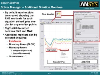
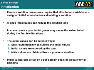
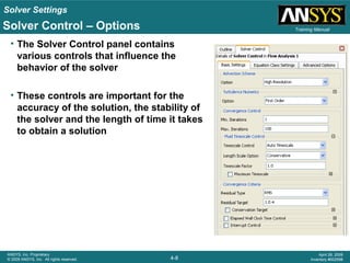
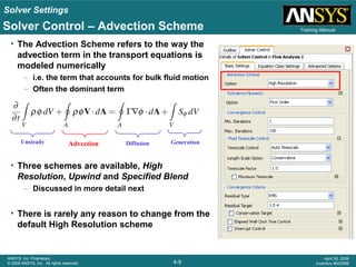
This document discusses various solver settings in ANSYS CFX that can be adjusted to control the behavior and performance of the computational fluid dynamics (CFD) simulation. It describes initialization methods for assigning initial conditions throughout the domain, as well as options in the solver control panel for settings like the advection scheme, convergence criteria, timescales and more. Guidance is provided on selecting appropriate values for key settings to achieve converged, accurate solutions in a timely manner.
![Solver Settings
4-21
ANSYS, Inc. Proprietary
© 2009 ANSYS, Inc. All rights reserved.
April 28, 2009
Inventory #002598
Training Manual
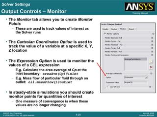
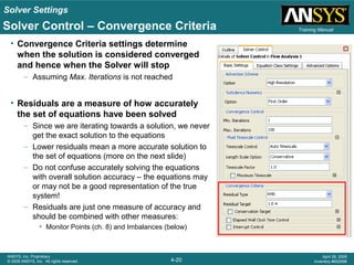
• The continuous governing equations are discretized into a set of linear
equations that can be solved. The set of linear equations can be written in
the form:
[A] [Φ] = [b]
where [A] is the coefficient matrix and [Φ] is the solution variable
• If the equation were solved exactly we would have:
[A] [Φ] - [b] = [0]
• The residual vector [R] is the error in the numerical solution:
[A] [Φ] - [b] = [R]
• Since each control volume has a residual we usually look at the RMS
average or the maximum normalized residual
Solver Control – Residuals Theory](https://image.slidesharecdn.com/cfx1204solver-150404102016-conversion-gate01/85/Cfx12-04-solver-21-320.jpg)
![Solver Settings
4-24
ANSYS, Inc. Proprietary
© 2009 ANSYS, Inc. All rights reserved.
April 28, 2009
Inventory #002598
Training Manual
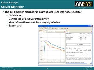
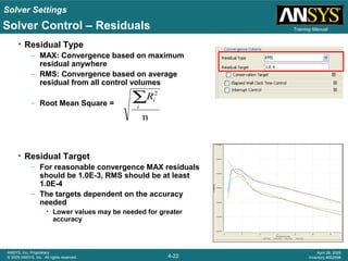
• Elapsed Time Control
– Can specify the maximum wall clock time
for a run
– Solver will stop after this amount of time
regardless of whether it has converged
• Interrupt Control
– Can specify other criteria for stopping
the Solver based on logical CEL
expressions
– When the expression returns true the
solver will stop
• Any value >= 0.5 is true
Solver Control – Elapsed Time and Interrupt Control
– Examples
• If temperature exceeds a specified value
if(areaAve(T)@wall>200[C],1,0)
• If mesh quality drops below a specified value in a moving mesh case
– More on logical expressions in the CEL lecture](https://image.slidesharecdn.com/cfx1204solver-150404102016-conversion-gate01/85/Cfx12-04-solver-24-320.jpg)