This document outlines the key steps in a typical computational fluid dynamics (CFD) analysis:
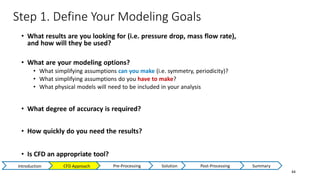
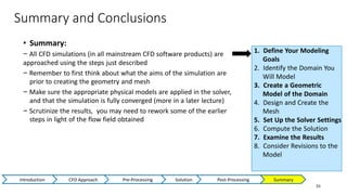
1) Define modeling goals and assumptions
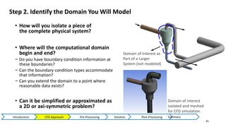
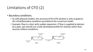
2) Identify the domain to be modeled
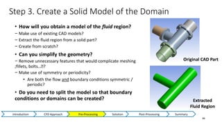
3) Create a geometric model of the domain
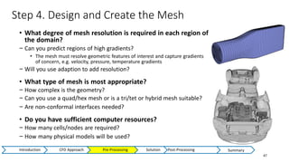
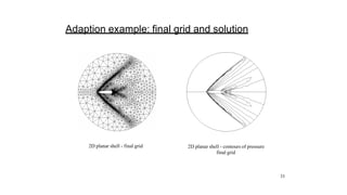
4) Design and create a mesh of the domain
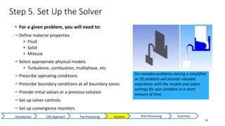
5) Set up the solver with appropriate physical models and boundary conditions
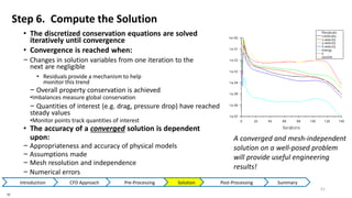
6) Compute the solution by solving the governing equations
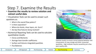
7) Examine the results to validate the solution and extract useful data