The document presents a design for a compressive light field camera that can recover high-resolution light fields from a single image, leveraging overcomplete dictionaries and optimized projections. It discusses the advantages of this approach, including improved image quality, while also addressing limitations such as reduced light transmission and increased capture time. Various applications of the technology, such as light field compression and denoising, are explored, highlighting its potential in the field of computational photography.

1. Compressive Light Field Photography using Overcomplete Dictionaries and Optimized Projections
ANKIT THIRANH
2011CS10210
ABSTRACT
In the previous two decades, light field photography has become one of the significant research interest. In this paper, a design is proposed for a compressive light field camera which will allow to recover light fields with higher resolution from a single image. Also, various other useful applications for light field atoms are discussed, including 4D light field compression and denoising.
Keywords
Computational photography, light fields, compressive sensing.
1. INTRODUCTION
In today world, cameras have become a really important part of our daily life. With the invention of digital mobile phones, anyone can click, edit and share their moments with anyone. Recently, in order to increase the level of quality of images, light field photography was introduced to market. It has various good features such as digital refocus and digital refocusing capabilities.
A computational light field camera has been proposed in this paper which has a unique feature of reconstruction of high resolution light fields from a single coded camera image. The architecture that is proposed contains three main components. First component is light field atom which is fundamental building block of natural night fields. Second is reconstruction of high-resolution light fields from a single coded projection. Finally, third is the optimization of optical system to provide incoherent measurements.
1.1 Advantages and Contributions
At first, exploration of light field photography was done and then, various parameters were calculated like optical and computational design patterns. Various new fields were introduces like light field atoms which are very important features of natural light fields. New compressive light field camera is built successfully.
1.2 Limitations
The proposed strategy sacrifices light transmission during capture process as it needs mask between sensor and camera lens. Also, it has increased access time as compared to previous light field cameras.
2. RELATED WORK
2.1 Light File Acquisition
The first work in field of Light Field Acquisition was done by (IVES H. , 1903) and (Lippman, 1908).They were the first of the persons who discovered the fact that light field inside a camera can be recorded. This feature has been integrated into digital cameras. (LUMSDAINE, 2009) and (GEORGIEV, 2006) have proposed alternative designs design that favor spatial resolution over angular resolution. Almost all of the above works were not able to fully preserve the image resolution. In order to preserve full image resolution, current proposals take multiple photographs with a single camera or include camera arrays. This paper describes a compressive light field camera design that recover a high resolution light field by taking only a single photograph.
2.2 Compressive Computational Photography
(WAKIN, 2006), (MARCIA, 2008), and (REDDY, 2011) applied compressive computational photography to discover video acquisition and then (PEERS, 2009) and (S EN, 2009)applied this to light transport acquisition. This paper proves that mask-based camera are better suited for compressive light field sensing.
This paper demonstrates that the light field atoms which are stored in over-complete dictionaries represent natural light fields more sparsely than previous methods. This paper proves that mask based approaches provide a good tradeoff between expected reconstruction quality and optional light efficiency. Finally, this paper shows how from a mask-modulated sensor image, we can recover a 2D photograph.
3. STEPS IN LIGHT FIELD CAPTURE AND SYNTHESIS
3.1 Acquiring Coded light field projections
This paper describes any image in the form i(x) captured by a camera. This image is projection of spatial-angular light filed represented by I(x,ν) along its angular dimension ν over the aperture area given by :
푖(푥)= ∫퐼(푥,휈)푑휈 휈 (1)
Where x is the two dimensional spatial dimension on the sensor plane and ν denotes the two dimensional position on the aperture plane at a distance da. Then, they propose to insert a coded attenuation mask f(ξ) at some distance dt from the sensor, which gives a new equation described as follows:
푖(푥)=∫푓(푥+푠(푣−푥))푙(푥,푣)푑푣 (2)
Where s= dt / da is defined as the shear of the mask pattern with respect to the light field. The coded light field projection can also be expressed in discretized form as:
i = ϕl, ϕ= [ϕ1 ϕ2 …… ϕpv2], (3)
where i ϵ ℝm and I ϵ ℝn are the vectorized sensor images and light field, respectively.
The observed image 푖= Σ흓풋푰풋풋 sums the light field views, where each view is multiplied by the identical mask code but is sheared by different amounts. The position of the mask plays a very useful role here. If the mask is situated directly on the sensor, this implies s=0, and therefore, the views are averaged. If the position of the mask is on the aperture, i.e., s=1, this will finally result in weighted averages of all light field views. However, the sampling happens when is mask is located in between sensor and aperture.

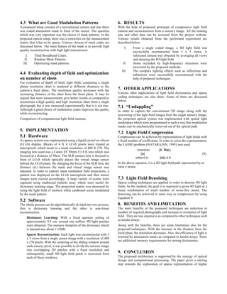
2. 3.2 Reconstructing Light Fields from Projections
It is just the inverse of linear system of equations (Eq. 3). For a single sensor image, the number of unknowns are significantly larger than the number of measurements, i.e., n>>m. An assumption is taken that natural light fields are sufficiently compressible in some kind of dictionary Ɗ ϵ ℝnXd, such that
i = ϕl = ϕ Ɗα, (4)
(CANDES`, 2008) and (DONOHO, 2006) gave a solution to the equation (4) on the basis that most of the coefficients in α ϵ ℝd have values approaching to zero. The solution provided is as follows:
minimize ||α||1 {α} (5) subject to ||i - ϕƊα||2 ≤ ϵ
which is known as pursuit denoise(BPDN) problem. In general, the Lagrangian formulation of Equation (5) is calculated. Based on the assumption that the light field can be well represented by a linear combination of at most k columns in Ɗ, a lower bound on the required number of measurements was calculated which comes out to be O(k log(d/k)).
The two main challenges for compressive computational photography are:
1) Knowledge of o “good” sparsity basis.
2) Scaling up of the reconstruction times to high resolutions.
Figure 1: Visualization of light filed atoms in an over-complete dictionary.
3.3 Learning Light Field Atoms
The learning of the light field atoms in over-complete dictionaries is proposed in the paper. A 4 dimensional spatio-angular light field patches of size n = px x px x pv x pv is considered and given a large number of training light fields, a dictionary Ɗ ϵ ℝnXd is learned as
Minimize ||L – Ɗ A||
{Ɗ, A} ∀j, ||αj||0 ≤ k (7) subject to
where L ϵ ℝn x q is taken as a training set which is comprised of q light field patches and A = [α1,….., αn] ϵ ℝnXq is a set of k-sparse coefficient vectors. The number of non-zero elements in an vector are counted by using Frobenius matrix which is given by
||X||2 = Σxij푖푗 (8)
Generally, training sets for the dictionary learning are extremely large and there are lot of redundancy and solving the equation is very expensive computationally
4. ANALYSIS
The structure of light field atoms and dictionaries are analyzed in this section. Also, evaluation of the proposed camera architecture is done along with its comparison with a range of alternative light field cameras.
4.1 Interpreting Light Field Atoms
The columns of each over-complete dictionary are designed to sparsely represent the complete training set and therefore capture the essential atoms. Also, as we can clearly see that the structure of these building blocks depends on the training set. Some people might think that there will be a lot of redundancy as the dimensionality is increased from 2D atoms to 4D light fields but the dimensionality gap is a 3D manifold in 4D light space, hence this model diffuse objects within a certain depth range.
4.2 Evaluation of Dictionary Design Parameters
 Size of light Field Atom: A general rule must always be followed for number of measurements m that m ≥ O (k log (d/k)). In this equation, m grows linearly with atom size, but the right side will only grow logarithmically as d is directly proportional to n. Also, there will be a decrease in the compressibility of the light field because there will be reduction in the local coherence within the atoms.
 Dictionary Overcompleteness: The over completenesss for the dictionaries is also calculated. In this, an estimate is calculated that how many atoms should be taken from a given training set. There came an observation that with the increase in the size of the dictionary, the redundancy grows as well.
Figure2: Evaluating dictionary completeness.

3. 4.3 What are Good Modulation Patterns
A proposed setup consists of a conventional camera and also there was coded attenuation mask in front of the sensor. The question which was very important was the choice of mask patterns. In the proposed optical setup, there was a restriction on the measurement matrix that it has to be sparse. Various choices of mask codes are discussed below. The main feature of the mask is to provide high quality reconstruction with high light transmission.
I. Tiled Broadband Codes.
II. Random Mask Patterns.
III. Optimizing mask patterns.
4.4 Evaluating depth of field and optimization on number of shots
For evaluation of depth of field, light fields containing a single planar resolution chart is rendered at different distances to the camera’s focal plane. The resolution quality decreases with the increasing distance of the chart from the focal plane. It may be argued that more measurements give better results as compared to reconstruct a high quality and high resolution chart from a single photograph, but it was measured experimentally that it is not true. Although a good choice of modulation codes improves the quality while reconstructing.
Comparison of computational light field cameras.
5. IMPLEMENTATION
5.1 Hardware
A capture system was implemented using a liquid crystal on silicon (LCoS) display. Blocks of 4 X 4 LCoS pixels were treated as macropixels which result in a mask resolution of 480 X 270. The imaging lens used was a Canon EF 50mm f/1.8 II lens which was focused at a distance of 50cm. The SLR camera lens is focused in front of LCoS which optically places the virtual image sensor behind the LCoS plane. By changing the focus of the SLR lens, the distance (d1) between the mask and virtual image sensor was adjusted. In order to capture mask modulated field projections, a pattern was displayed on the LCoS macropixels and then sensor images were resized accordingly. A large variety of scenes were captured using traditional pinhole array which were useful for dictionary learning stage. The projection matrix was measured by using the light field of uniform white cardboard scene modulated by the mask pattern.
5.2 Software
The whole process can be algorithmically divided into two process, first is dictionary learning and the other is non-linear reconstruction.
Dictionary Learning: With a fixed aperture setting of approximately 0.5 cm, around one million 4D light patches were obtained. The memory footprint of the dictionary which is learned was about 111MB.
Sparse Reconstruction: Each light was reconstructed with 5 x 5 views from a single sensor image with a resolution of 480 x 270 pixels. With the centering of the sliding window around each sensory pixel, it was possible to divide the sensory image into overlapping 2D patches with a fixed resolution and subsequently, small 4D light field patch is recovered from each of these windows.
6. RESULTS
With the help of proposed prototype of compressive light field camera and reconstruction from a sensory image. All the training sets and other data can be accessed from the project website. Various results obtained from the performed experiment are described below:
I. From a single coded image, a 4D light field was successfully reconstructed from 5 x 5 views. A refocused camera was obtained by averaging all views and shearing the 4D light field.
II. Areas occluded by high-frequency structures were recovered by the proposed methods.
III. The complex lighting effects such as reflections and refractions were successfully reconstructed with the help of proposed techniques.
7. OTHER APPLICATIONS
Various other applications of light field dictionaries and sparse coding techniques are also there. Some of them are discussed below.
7.1 “Undappling”
In order to capture the conventional 2D image along with the recovering of the light field images from the single sensory image, the proposed optical system was implemented with spatial light modulators which were programmed in such a way that modulation masks can be mechanically removed out of the optical path.
7.2 Light Field Compression
Compression can be achieved by representation of light fields with a fixed number of coefficients. In order to solve this representation, the LASSO problem (NATARAJAN, 1995) was used
minimize ||I- Ɗα||2 {α} (9) subject to ||α||0 ≤ k
In the above equation, I is a 4D light field path represented by at most k atoms.
7.3 Light Field Denoising
Sparse coding techniques are applied in order to denoise 4D light fields. In this method, the goal is to represent a given 4D light as a linear combination of small number of noise-free atoms. The denoising can be achieved in same way as compression by using Equation 9.
8. BENEFITS AND LIMITATION
The main benefits of the proposed techniques are reduction in number of required photographs and increase in resolution of light field. They are less expensive as compared to other techniques such as lenslet arrays.
Along with the benefits, there are some limitations also for the proposed techniques. With the increase in the distance from the focal plane, the resolution decreases. Also, the efficiency of light is lowered by attenuation masks as compared to lenslet arrays. There are additional memory requirements for storing dictionaries.
9. CONCLUSION
The proposed architecture is supported by the synergy of optical design and computational processing. The paper gives a starting step towards the exploration of sparse representation of higher

4. dimensional visual signals. New techniques have to be devised for the improvement of the computational methods for data analysis and reconstruction.
10. REFERENCES
1) CANDES`, E. A. (2008). An Introduction to Compressive Sampling. IEEE Signal Processing 25, 2, 21–30.
2) DONOHO, D. (2006). Compressed Sensing. IEEE Trans. Inform.
3) GEORGIEV, T. A. (2006). Spatio-angular Resolution Tradeoffs in Integral Photography. EGSR, 263–272.
4) HITOMI, Y. G. (2011). Video from a Single Coded Exposure Photograph using a Learned Over-Complete Dictionary. IEEE ICCV.
5) IVES, H. (1903). Parallax Stereogram and Process of Making Same. US.
6) Lippman, G. (1908). La Photographie Integrale. Academie desSciences 146, 446–451.
7) LIPPMANN, G. (1908). La Photographie Integrale. Academie des Sciences 146, 446–451.
8) LUMSDAINE, A. A. (2009). The Focused Plenoptic Camera. Proc. ICCP, 1–8.
9) MARCIA, R. F. (2008). Compressive coded aperture video reconstruction. EUSIPCO.
10) NATARAJAN, B. K. (1995). Sparse Approximate Solutions to Linear Systems. SIAM J. Computing 24, 227–234.
11) PEERS, P. M. (2009). Compressive light transport sensing. ACM Trans. Graph. 28,3.
12) REDDY, D. V. (2011). Programmable Pixel Compressive Camera for High Speed Imaging. IEEE CVPR, 329–336.
13) S EN, P. A. (2009). Compressive dual photography. Computer Graphics Forum 28, 609–618.
14) WAKIN, M. B. (2006). Compressive imaging for video representation and coding. . Picture Coding Symposium.