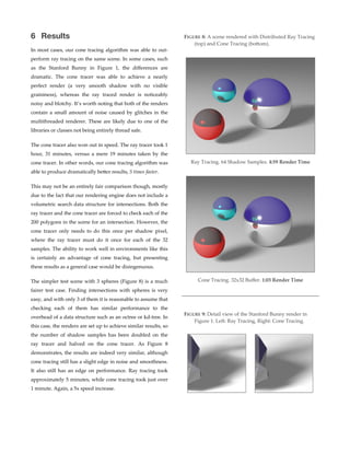
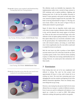
This document discusses a method called cone tracing, which is a variant of ray tracing that can be used to render realistic soft shadows and glossy reflections more efficiently than traditional ray tracing. The key aspects are: - Cone tracing models light as conical volumes rather than individual rays, reducing the number of intersections needed while avoiding noise. - The paper presents a rendering engine that uses both cone tracing and ray tracing modules to produce shadows and reflections. Cone tracing is used to determine occlusion and reflection colors at ray intersection points. - Intersection algorithms are approximated for cones, which have linear widening, rather than solved directly through systems of equations like with rays. This achieves accurate results more efficiently

1. Rendering Soft Shadows and Glossy Reflections with Cone Tracing
Keaton Brandt – brandk7@rpi.edu
FIGURE 1: A 200 polygon Stanford Bunny with soft shadows rendered using traditional ray tracing (left, 32 shadow samples) and
cone tracing (right, 64x64 cone buffer resolution).
Abstract
In this paper we demonstrate a method of rendering scenes
using cone tracing, a variant of ray tracing. Specifically, we
use cones to render realistic shadows from non-­‐‑point light
sources (soft shadows), and to simulate reflections from
surfaces that are not perfect mirrors (glossy reflections).
These effects are possible with traditional ray tracing, but
require a great deal of compute power to get good results.
Our cone tracing algorithm is able to out-­‐‑perform ray
tracing in most scenarios.
1 Introduction
Ray tracers model light using infinitely thin straight lines,
which results in a relatively accurate physical simulation of
photons but requires massive oversampling of the scene in
order to produce clean results. To render things like soft
shadows and glossy reflections, ray tracers ‘distribute’
single beams into dozens or even hundreds of secondary
beams that emanate outwards from intersection points.
Cone tracing simplifies this step by modeling these
secondary rays as a single volumetric cone shape that can
be intersected with the scene geometry. In other words,
instead of modeling the actual straight-­‐‑line photons, the
renderer models the entire region in which those photons
could potentially exist.
Such a system has two major advantages. First, it speeds up
rendering by reducing the number of intersections that
need to be calculated. Second, it does not involve any
randomness and therefore reduces the amount of noise in
the scene. It can, theoretically, replicate any effect currently
accomplished with distributed ray tracing.
The biggest downside is that it adds a huge amount of
complication to the rendering engine, which makes the
software harder to extend and optimize. It can also be very
difficult to debug due to the number of sub-­‐‑systems
involved (cone intersection, scan-­‐‑line conversion, cone
generation, geometry division, etcetera). For these reasons,
cone tracing is rarely used in production environments.
However, Occam’s Razor is not an immutable law of the
universe; sometimes more complicated solutions are more
effective than simpler ones. For this reason, we believe that

2. cone tracing should be revisited, and have demonstrated
that it can work alongside ray tracing to produce fast,
excellent results in a wide variety of situations.
1.1 Prior Work
Cone tracing was first proposed in “Ray Tracing with
Cones” [Amanatides 1984]. The paper outlines the basic
concept and a variety of approximate intersection
algorithms. The results are particularly impressive for 1984,
however he does not compare them to traditional ray
tracing for quality or speed. His system also models
everything as cones, even in situations where rays would
suffice and be faster. Still, it is easily the foundational paper
of the field, and most of the algorithms in this paper are
based off of his work.
A similar method, beam tracing, was proposed the same
year in “Beam Tracing Polygonal Objects” [Heckbert &
Hanrahan 1984]. It is a similar concept, but it uses
rectangular prism or square pyramid shapes instead of
circular cones. Their work involved optimizing non-­‐‑glossy
reflection and refraction by taking advantage of the spacial
coherence of a scene using a ‘beam tree’, instead of the
traditional recursive approach to ray tracing. The paper
provides a much more detailed approach to fast CPU-­‐‑based
scan conversion of polygons that acempts to minimize gaps
between shapes.
The beam tracing approach is expanded to handle scene
antialiasing in “A Beam Tracing Method with Precise
Antialiasing for Polyhedral Scenes” [Ghazenfarpour &
Hasenfraf, 1998]. Their method is able to work on any
convex polyhedra, and includes many optimizations not
possible for more complex scenes. They also briefly explore
applying these same optimizations to soft shadows, and
compare those results to traditional ray tracing. They were
the first to prove that volumetric samples (beams or cones)
can be more computationally efficient than rays.
Cone tracing has not achieved widespread adoption,
however with the advent of programmable GPUs there has
been a resurgence of interest in the topic. For example,
“Interactive Indirect Illumination Using Voxel Cone
Tracing” [Crassin et. al. 2011] explores its use as a way to
achieve effects such as radiosity in real time on the GPU (it
was co-­‐‑sponsored by Nvidia). They do this by representing
the scene as a grid of cubic ‘voxels’, rather than polygon
meshes or surface geometry. This modern research proves
that cone tracing is worth revisiting, and that its usefulness
may actually extend beyond what distributed ray tracing is
capable of.
2 Approach
This paper describes a system capable of using both rays
and cones to render a scene. The rendering of each pixel
starts with a ray being cast outwards from the camera.
When that ray hits an object, the ray tracer calls on the cone
tracer to determine the shadow and reflection colors at the
intersection points, and factors those results into those final
color calculations for the pixel. The cone tracer can also call
itself to create tertiary cones for reflections and shadows
inside of reflections. This modular system, diagrammed in
figure 2, lays out a clear separation of concerns for the
different classes.
FIGURE 2: A high-­‐‑level view of the architecture of the
dual-­‐‑mode rendering engine.
Render Thread
Ray Tracer
Shadow Occlusion
Cone Tracer
Reflection
Cone Tracer
Pixel Location Pixel Color
% Occlusion
Point, Normal Reflection
Color
Point, Light
Reflection Intersection Point -­‐‑> % Occlusion

3. The cone tracer itself is broken up into several different
modules. The core class creates cone objects, lists and sorts
their intersections with objects in the scene, and then has
the cone buffer class determine a ‘cones eye view’ and
average the results. The cone-­‐‑object intersection algorithms,
discussed in detail in section 3, are included in the
representative classes for each object to allow for easy
extension. The cone buffer class includes a scan-­‐‑line
renderer that works for circle, plane and polygon shapes,
and can draw either greyscale or color data. Each
component can be debugged individually, which goes a
long way towards addressing the complexity problems.
The ray tracing class can also be toggled to use distributed
ray tracing instead of cone tracing. That system includes
stratified sampling to reduce noise. Scene-­‐‑wide antialiasing
is also accomplished using distributed ray tracing. The
rendering engine does not include a volumetric data
structure such as a k-­‐‑d tree for faster intersection lookup,
which dramatically slows down scenes with a large number
of polygons.
2.1 Cone Representation
The cone representation class is a simple extension of a
standard ray representation, which includes an origin point
and a direction vector. Cones are modeled as rays with a
non-­‐‑zero width that changes linearly with the distance
along the ray. In other words, the radius of the cone is
represented as a linear equation:
Where t is a parameter distance along the center line of the
cone. Because all cones use this linear function, their width
can be represented with only the spread coefficient, h.
Therefore, cones can be entirely modeled by two vectors
(origin and direction) and one scalar (h).
3 Intersection Algorithms
Determining intersections between 3D shapes and cones is
a licle more challenging than using rays. For one thing, ray-­‐‑
object intersections always result in a finite number of
points, of which the closest one can be chosen. Cone-­‐‑object
intersections generally result in 3D lines, generally modeled
using cubic equations. As a result, direct system-­‐‑of-­‐‑
equations solutions are inefficient and unnecessary. Instead,
a number of different approximations are used, which
achieve accurate results in most situations.
3.1 Cone-Sphere Intersection
If it is assumed that the entirety of the sphere is in front of
the cone’s origin point, intersections can be determined by
simply finding the shortest distance from the center point of
the sphere to the center ray of the cone. An intersection
exists if this distance, d, is less than the sum of the radius of
the sphere and the radius of the cone at that point. Figure 3
demonstrates this graphically.
Finding d first involves finding a plane orthogonal to the
center line of the cone that includes the center point of the
sphere.
Where is the center point of the sphere and is the
direction vector of the cone. The plane is defined implicitly,
so finding the distance from the origin point of the cone to
the plane (the t parameter) is a simple macer of algebra.
Knowing t is not only useful for determining the radius of
the cone, it also means that d can be calculated using the
pythagorean theorem.
Where c is the origin point of the cone. The cone and sphere
intersect if and only if d < cr + r(t). Center Ray
Origin
r(t)
t

4. 3.2 Cone-Polygon Intersection
Finding the actual 3D intersection between a cone and an
arbitrary polygon is a very complicated problem. It is also a
very common problem, since 3D models are usually treated
as collections of triangles or quads. Luckily, it can be
reduced to a 2D problem using the same perspective
transformations that simulate cameras [Amanatides 1984].
In other words, instead of dealing with each point of the
polygon in 3D space, each point is mapped to a 2D location
in the “cone’s eye view” and the intersection algorithm
operates on that.
The transformation matrix is calculated the same way as it
would be for a camera. The focal length, f, is equal to 1/h.
The near clipping plane is set as close to zero as possible
without encountering floating point error, and the far plane
is set to infinity. With only these variables, an intrinsic
camera matrix can be created.
This matrix can then be multiplied by rotation and
translation matrices to fully represent the point of view of
the cone. Then 3D points can be mapped onto the cone’s 2D
viewport by multiplying them by the transformation
matrix. A point that lies on the cone’s center line will map
to (0,0). Any point whose distance from (0,0) is less than 0.5
is considered to be within the circular viewport.
Even with the points reduced to 2D, several cases have to be
considered when checking for intersections.
3.2.1
Vertex in View
The simplest, and most common, case occurs when one of
the vertices of the polygon is within view of the cone. If the
cone can see a vertex, it can obviously see the shape.
3.2.2
Cone Center inside Polygon
If a polygon blocks the entire view of the cone, none of its
points will be within the viewport. To detect this situation,
2D ray casting is used. If every ray passing from the center
of the viewport through one of the edges of the polygon
intersects an odd number of edges, the circle is inside the
polygon. An even number of intersections means the ray
both entered and exited the polygon, which means that it
was not inside the shape to begin with. This is the most
compute intensive check, so it is performed last.
3.2.3
Edge Intersection
Even if both of those tests fail, there could still be an
intersection. As Figure 4 demonstrates, it is possible to have
an edge of the polygon intersect with an edge of the
viewport. These intersection points can be found using a
similar method to the sphere intersection algorithm
described in Section 3.1. The code finds the closest point on
the edge to (0,0), the center of the viewport. If the point is
closer than 0.5 units away, there is an intersection.
FIGURE 3: A 2D diagram representing the logic behind
cone-­‐‑sphere intersection. The left cone has an
intersection, the right one does not.
d
cr
r(t)
d
cr
r(t)
FIGURE 4: Different types of cone-­‐‑triangle intersections.
Vertex in View Cone Center Inside
Edge Intersection

5. 3.3 Cone-Plane Intersection
The third intersection algorithm came in handy for the
simple test scenes used in this paper, but is less common in
production applications. It models a plane that extends
infinitely in all directions, which is useful in part because it
is so easy to find intersections.
The sine of the angle between the center of the cone and the
normal vector of the plane is determined using a dot
product. The sine of the spread angle of the cone is also
determined as:
If the angle between the cone and the normal is less than
sin(π/2) -­‐‑ a then there is no intersection. If it is greater than
sin(π/2) + a then there is a full intersection (the plane fully
occludes the cone). The percent occlusion of the cone varies
linearly from sin(π/2) -­‐‑ a to sin(π/2) + a.
4 Scan-line Rendering
The viewpoint of each cone is rendered using a simple
CPU-­‐‑based scan-­‐‑line renderer. Only the average value of
this viewport actually macers, but it is important to draw
the shapes correctly in a 2D buffer because some objects
may partially or entirely occlude other objects.
To cut out the relatively costly averaging step at the end,
the renderer keeps a running total of every pixel in view.
Whenever a pixel is changed, the sum is updated. The soft
shadow cone tracer determines occlusion by comparing the
sum of the buffer after the light is drawn, and then again
after every object in front of the light is drawn. The light has
a value of 255 and the objects have a value of 0, so any
objects blocking the light will decrease the sum.
Every polygon shape can be reduced to triangles. Plane
intersections are represented as quads that face the correct
direction and occlude the correct amount of the view.
Therefore, only two scan-­‐‑line rendering algorithms are
needed for the buffer.
4.1 Circle Rendering
Scan-­‐‑line renderers are so named because they draw shapes
one line at a time. Therefore, scan-­‐‑line rendering of a circle
essentially boils down to figuring out where each line starts
and ends (because a circle has no holes in the middle).
Using the pythagorean theorem, it is easy to find the width
of a circle at a given y value above or below its center.
Where r is the radius of the circle and cy is the y component
of its center in viewport coordinate.
A line is drawn from xstart to xend for every scan-­‐‑line,
clipping both values to be within range of the buffer.
4.2 Triangle Rendering
Triangles are easy to render in scan-­‐‑lines when 2 of the
vertices are lined up on the y axis. These axis-­‐‑oriented
triangles can be rendered by simply interpolating the start
and end x values from the 2 aligned points to the 1 outlier
point. All triangles can be converted into axis-­‐‑aligned
triangles by splicing them in half. The split point passes
through the vertex with the median y-­‐‑value. Then, both
halves are rendered separately. Anti-­‐‑aliasing can be added
by blending pixels with non-­‐‑integer x or y values.
FIGURE 5: Scan-­‐‑line rendering process for triangles.

6. 4.3 Rendering Glitches
It was very difficult to achieve clean results due to the
number of different edge cases present when working with
complex 3D geometry. For example, when some points on
the polygon are behind the camera and some are in front,
the 2D mapping is unreliable. The algorithm currently does
not account for this problem (OpenGL solves it with
frustum culling).
Another problem is that floating point error causes triangles
to not perfectly line up, which often causes some scan-­‐‑line
to incorrectly be marked on or off. Two examples of this,
caused by slightly different phenomena, are shown in
Figure 6.
5 Reflections
Glossy Reflections proved to be a very difficult challenge,
mostly due to the difficulty of debugging them. Even
simple scenes can end up with dozens of reflections and
shadow cones per pixel, each contributing to one another in
non-­‐‑obvious ways. Figure 7 shows one such scene. For this
reason, we were never able to achieve desirable results from
cone-­‐‑traced reflections. However, much of the math behind
the reflection algorithm is solid, at least for the cases
examined by this paper.
5.1 Generating Secondary Reflection Cones
Secondary reflection cones are cones that are created when
a reflection cone intersects a reflective object. The secondary
cone must cover the entire intersection region, and reflect
across the normal of the intersection point. This is easy for
flat geometry that has only one normal and a clear
boundary for intersection. Spherical geometry is more
complicated, but can be approximated by simply taking the
normal at the center point of the intersection.
When reflecting off of flat, non-­‐‑glossy surfaces, the spread
value of the secondary cone remains the same. Glossy
surfaces will increase the spread value, since glossy objects
are able to reflect a slightly larger area of the scene. Curved
surfaces will also affect the spread value; Convex curves
will expand it, concave curves will decrease or even negate
it. Objects with both concave and convex regions will need
to be split into multiple shapes (this is beyond the scope of
the paper).
The intersection is represented with a circumcircle, a flat
circle that contains the entire intersection. A cone is then
created with the desired spread value that passes through
this circle. The t parameter of the cone is offset so that the
original circle is the cone’s slice at t=0. In other words, the
cone extends behind the intersection, but that part is
ignored.
FIGURE 6: Two examples of rendering bugs. Left: A
shadow cone buffer from the Stanford Bunny scene
showing horizontal line artifacts. Right: A shadow
buffer demonstrating poorly anti-­‐‑aliased lines.
FIGURE 7: A debugging view of all the cones created for a
single pixel, each represented by their center line.
Red = Reflection Cone. Blue = Shadow Cone.

7. 6 Results
In most cases, our cone tracing algorithm was able to out-­‐‑
perform ray tracing on the same scene. In some cases, such
as the Stanford Bunny in Figure 1, the differences are
dramatic. The cone tracer was able to achieve a nearly
perfect render (a very smooth shadow with no visible
graininess), whereas the ray traced render is noticeably
noisy and blotchy. It’s worth noting that both of the renders
contain a small amount of noise caused by glitches in the
multithreaded renderer. These are likely due to one of the
libraries or classes not being entirely thread safe.
The cone tracer also won out in speed. The ray tracer took 1
hour, 31 minutes, versus a mere 19 minutes taken by the
cone tracer. In other words, our cone tracing algorithm was
able to produce dramatically becer results, 5 times faster.
This may not be an entirely fair comparison though, mostly
due to the fact that our rendering engine does not include a
volumetric search data structure for intersections. Both the
ray tracer and the cone tracer are forced to check each of the
200 polygons in the scene for an intersection. However, the
cone tracer only needs to do this once per shadow pixel,
where the ray tracer must do it once for each of the 32
samples. The ability to work well in environments like this
is certainly an advantage of cone tracing, but presenting
these results as a general case would be disingenuous.
The simpler test scene with 3 spheres (Figure 8) is a much
fairer test case. Finding intersections with spheres is very
easy, and with only 3 of them it is reasonable to assume that
checking each of them has similar performance to the
overhead of a data structure such as an octree or kd-­‐‑tree. In
this case, the renders are set up to achieve similar results, so
the number of shadow samples has been doubled on the
ray tracer and halved on the cone tracer. As Figure 8
demonstrates, the results are indeed very similar, although
cone tracing still has a slight edge in noise and smoothness.
It also still has an edge on performance. Ray tracing took
approximately 5 minutes, while cone tracing took just over
1 minute. Again, a 5x speed increase.
FIGURE 8: A scene rendered with Distributed Ray Tracing
(top) and Cone Tracing (bocom).
Ray Tracing. 64 Shadow Samples. 4:59 Render Time
Cone Tracing. 32x32 Buffer. 1:03 Render Time
FIGURE 9: Detail view of the Stanford Bunny render in
Figure 1. Left: Ray Tracing, Right: Cone Tracing.

8.
The reflection results are decidedly less impressive. Our
implementation suffers from a myriad of bugs common to
GPU rendering, such as epsilon problems, z-­‐‑fighting, and
floating point error. It also has the problem discussed in
Section 5 where geometry with points on both sides of the
cone cannot be properly mapped into the cone buffer. This
leads to the bug demonstrated in Figure 11. This bug was
never fixed, which is why the scene in Figure 10 has an
infinite plane instead of a ground quad.
Figure 10 shows that our algorithm clearly needs more
work when it comes to glossy reflections. Most of the detail
is lost, and the elements that remain appear to be blown
out. There are also some even more basic bugs, such as the
reflection of the red sphere gecing randomly cut off on the
blue sphere (likely due to an incorrectly calculated z-­‐‑value
for the ground plane). Our implementation also does not
work with textured surfaces, and doing so would likely
slow it down significantly since the cone buffer would need
to sample the texture at each pixel.
Still, the cone tracer was able to produce at least slightly
accurate results in just 2.5% of the time it took the ray tracer
to produce grainy results. Even with the texture sampling
in place, it is likely that cone tracing could handily beat ray
tracing. However, we cannot prove that conclusively with
these results.
7 Conclusion
Cone tracing does turn out to be very complicated and
difficult to debug. The code for this project took
approximately 42 hours to write, and is based off of an
existing ray tracer. The most time consuming parts were
debugging the scan-­‐‑line renderer and figuring out all of the
different intersection algorithms. There are certainly many
more things that can go wrong.
However, cone tracing has also proven itself to be far more
efficient than ray tracing in a number of different scenarios.
Even if cones are used for nothing but soft shadows, it can
speed up a render by as much as 500%. With glossy
reflections working, that speed-­‐‑up could be even greater.
FIGURE 10: A glossy scene rendered with Distributed Ray
Tracing (top) and Cone Tracing (bocom).
Ray Tracing. 32 Glossy Samples. 05:24:52 Render Time
Cone Tracing. 32x32 Buffer. 00:08:04 Render Time
FIGURE 11: A bug that occurs when the cone traced scene
is placed on a non-­‐‑infinite ground plane

9. Although cone tracing was first proposed over 30 years ago,
there has been licle research. Optimizations in traditional
ray tracing have made it viable in most situations, so there
has not been much demand for a different strategy.
However, physically accurate real-­‐‑time rendering is starting
to become achievable thanks to the dramatic advances in
GPU technology over the past few years. Teams at
companies like Nvidia are starting to demonstrate ray
tracers that are capable of running entirely on the GPU.
These systems generally cannot scale up very well, partly
because of the difficulty of maintaining spacial data
structures for dynamic scenes, and partly due to
inefficiency inherent in the implementation.
Modern GPUs are programmable, but they have limits.
They are still designed around the traditional rendering
pipeline, so everything on top of that relies on hacks like
pucing data into textures. Many GPUs cap the size of
textures due to memory constraints, which in turn
constrains the size of the scene that can be processed. We
propose a hybrid method of real-­‐‑time rendering that uses
the CPU to generate rays and cones in a scene, and uses the
GPU to render the cone buffers using its normal pipeline.
Unfortunately, such an idea is well beyond the scope of this
paper, but it shows why research into cone tracing may be
important to the future of computer graphics.
8 References
AMANATIDES, J. 1984. Ray tracing with cones. In
Proceedings of the 11th Annual Conference on
Computer Graphics and Interactive Techniques,
ACM, New York, NY, USA, SIGGRAPH ’84,
129-­‐‑135.
CRASSIN, C., NEYRET, F., SAINZ, M., GREEN, S. AND
EISEMANN, E. 2011. Interactive Indirect
Illumination Using Voxel Cone Tracing. In
Computer Graphics Forum, 30, 1921–1930.
GHAZANFARPOUR, D. AND HASENFRATZ, J.M. 1998. A
Beam Tracing Method with Precise Antialiasing
for Polyhedral Scenes. Laboratoire MSI -­‐‑ Université
de Limoges.
HECKBERT, P. AND HANRAHAN, P. 1984. Beam tracing
polygonal objects. In Proceedings of the 11th Annual
Conference on Computer Graphics and Interactive
Techniques, ACM, New York, NY, USA,
SIGGRAPH ’84, 119-­‐‑127