This document provides an overview of digital signal processing concepts including sampling, quantization, pulse code modulation (PCM), delta modulation, and multiplexing techniques. It discusses the Nyquist sampling theorem and how analog signals are converted to digital through sampling, quantization, and encoding. PCM is described as converting analog signals to digital codes. Delta modulation and its use of oversampling and simple quantization is also covered. Finally, the document discusses digital multiplexing methods like time-division multiplexing (TDM) where multiple digital signals are allocated unique time slots within a common signal frame.

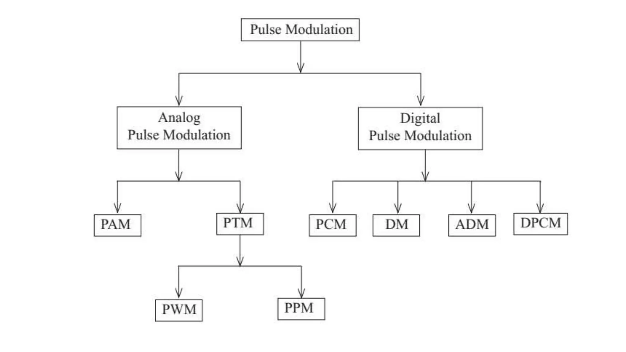
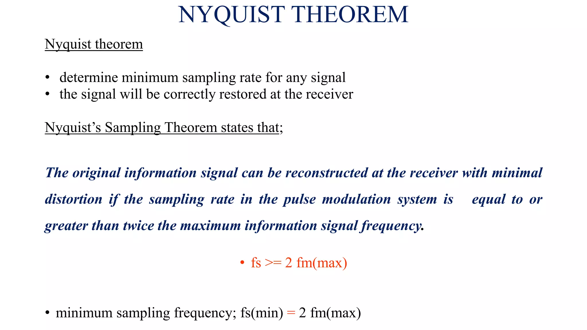
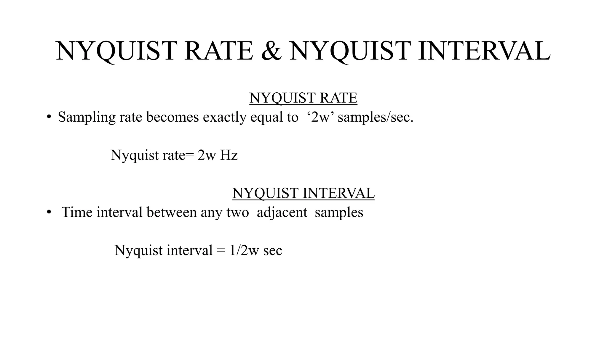
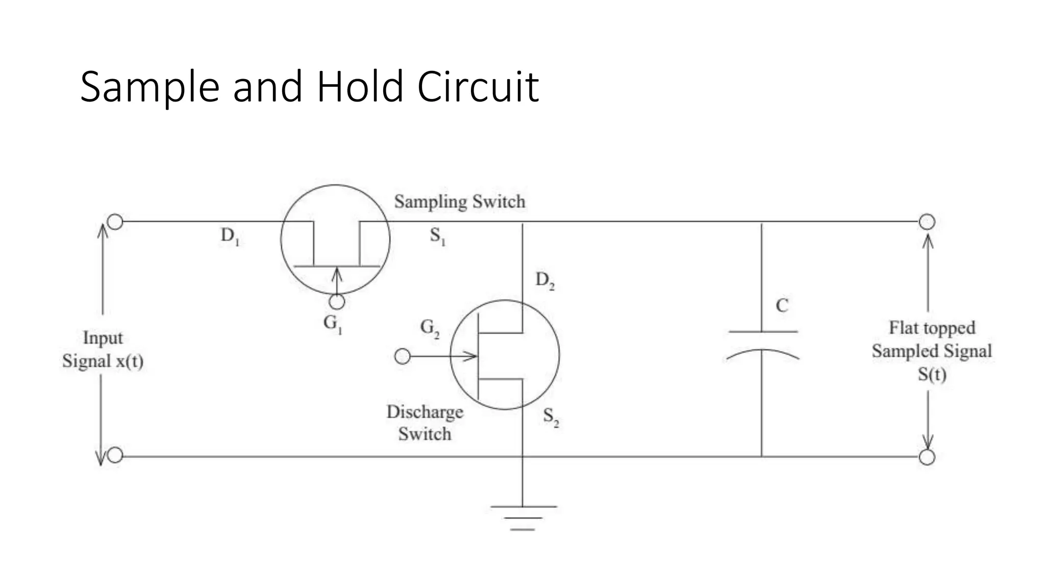
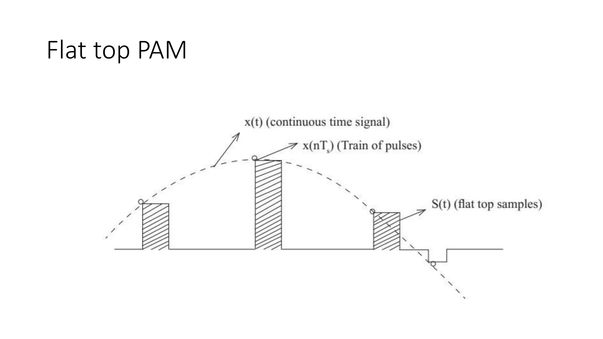
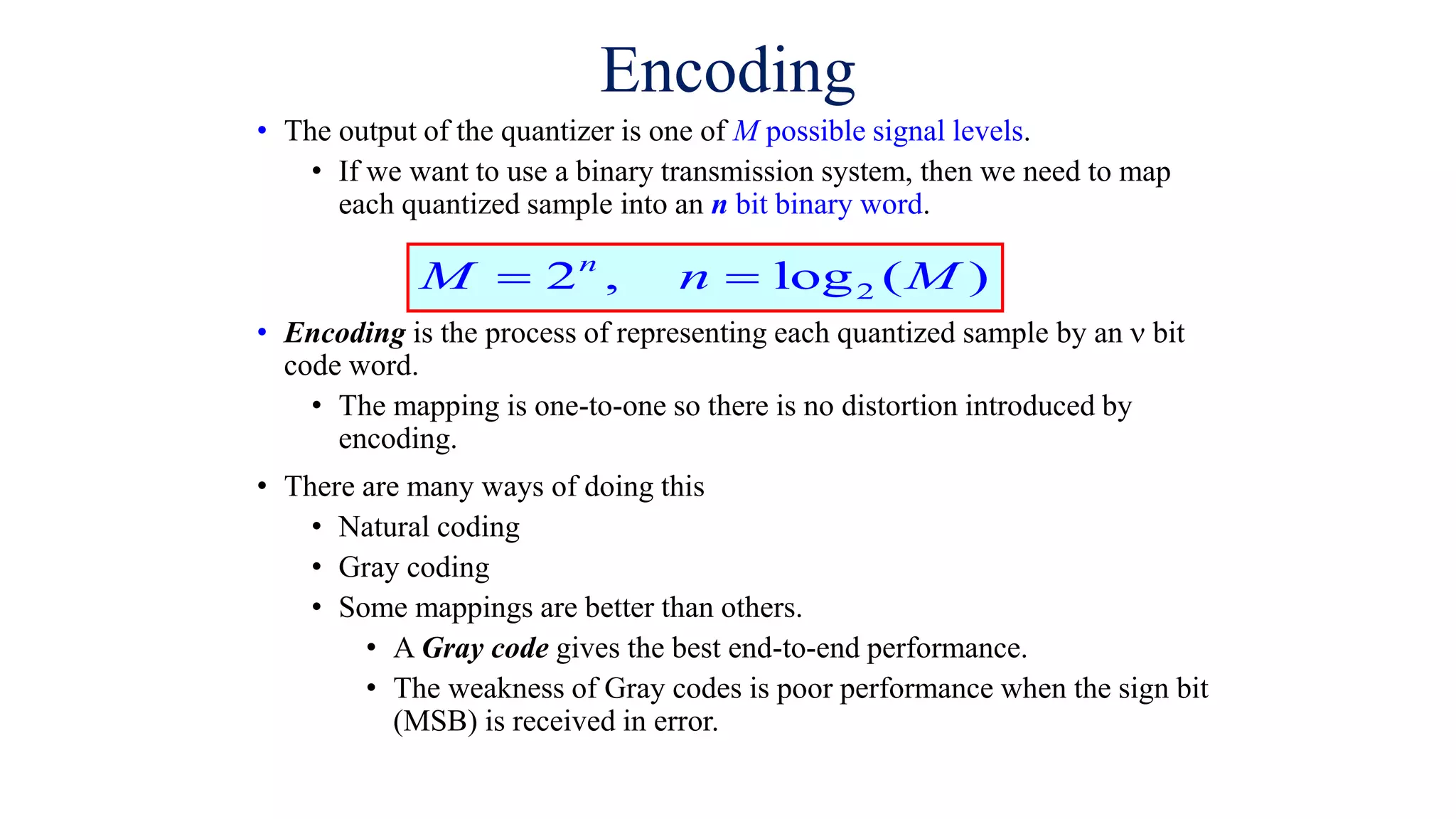
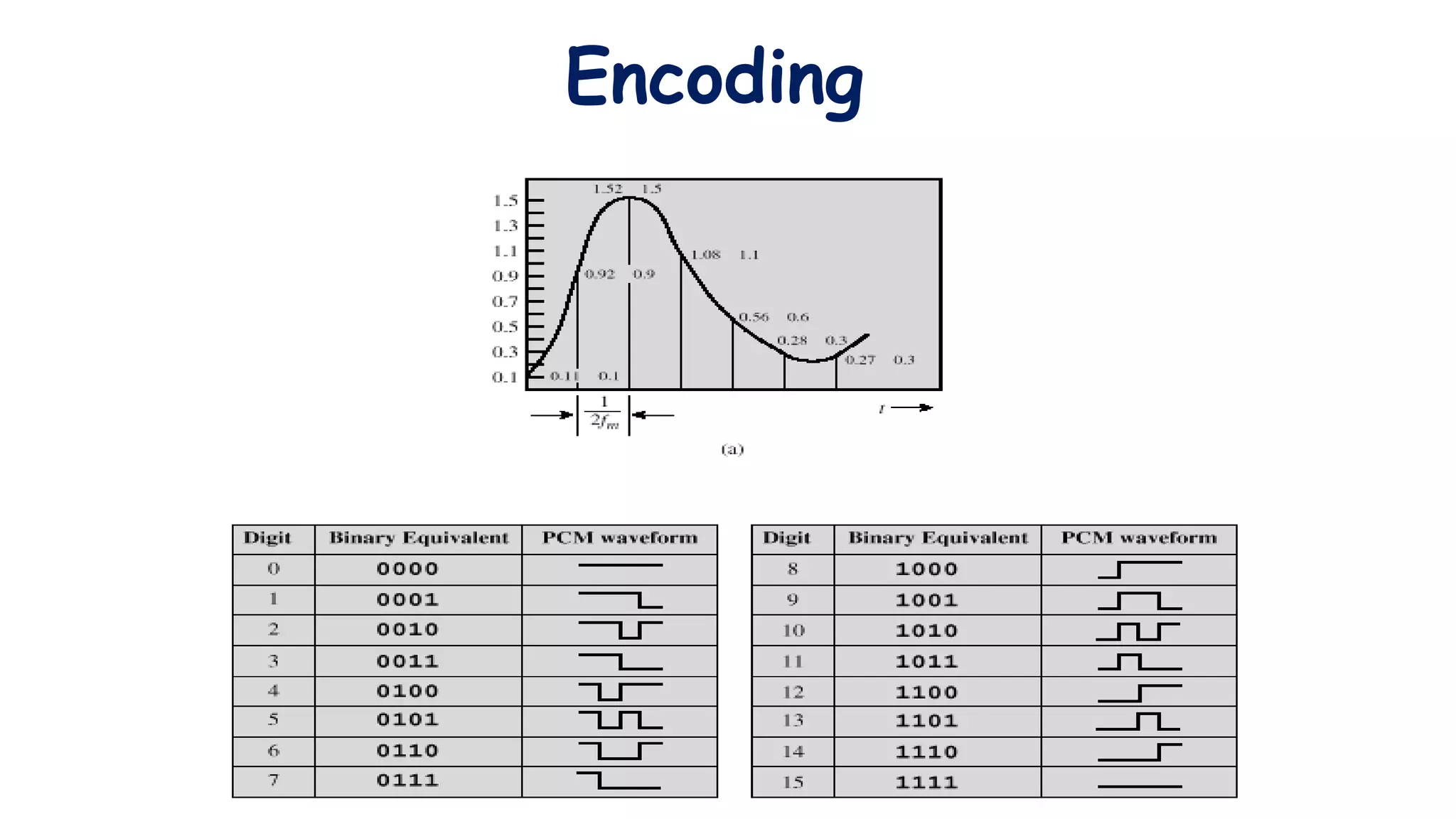
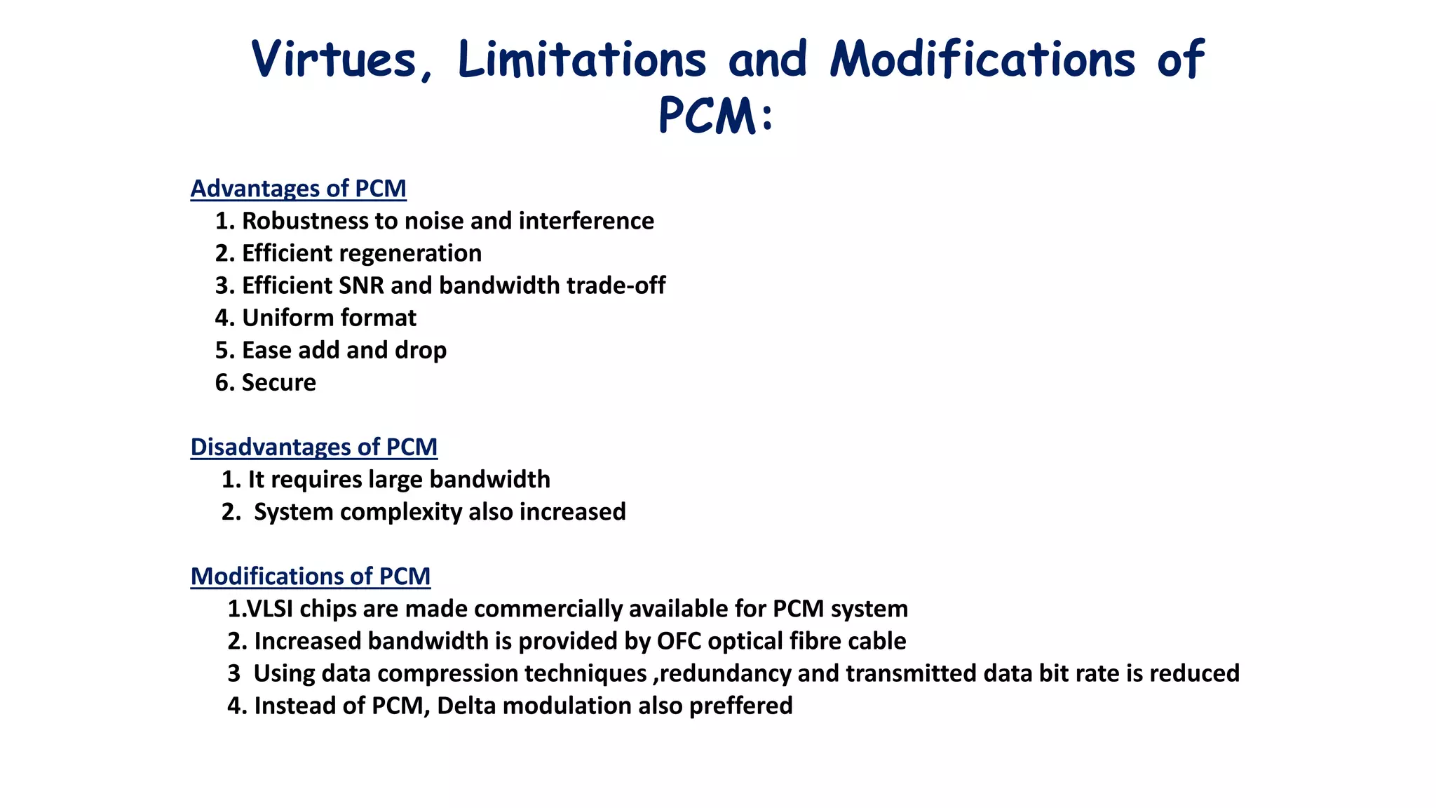
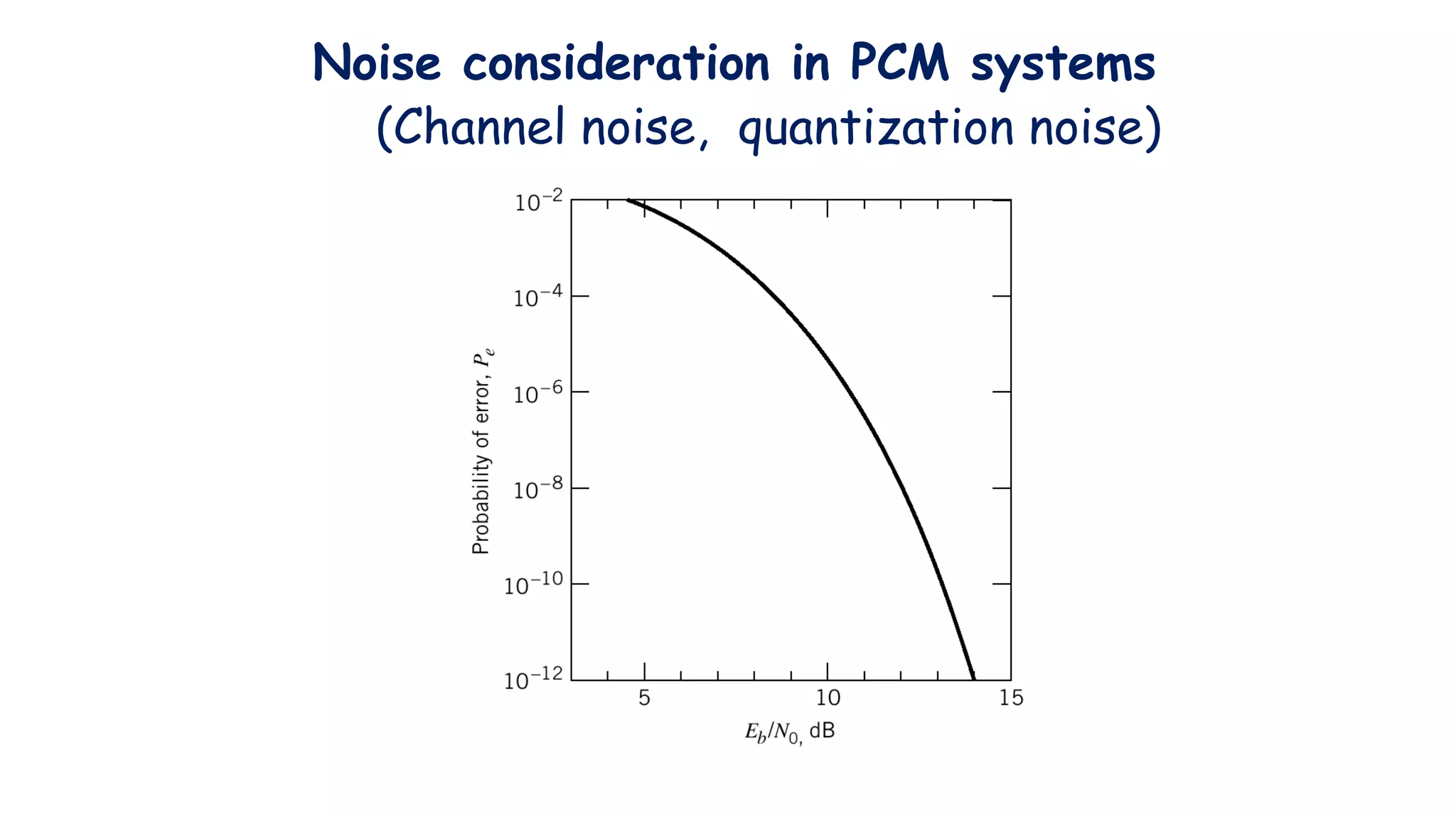
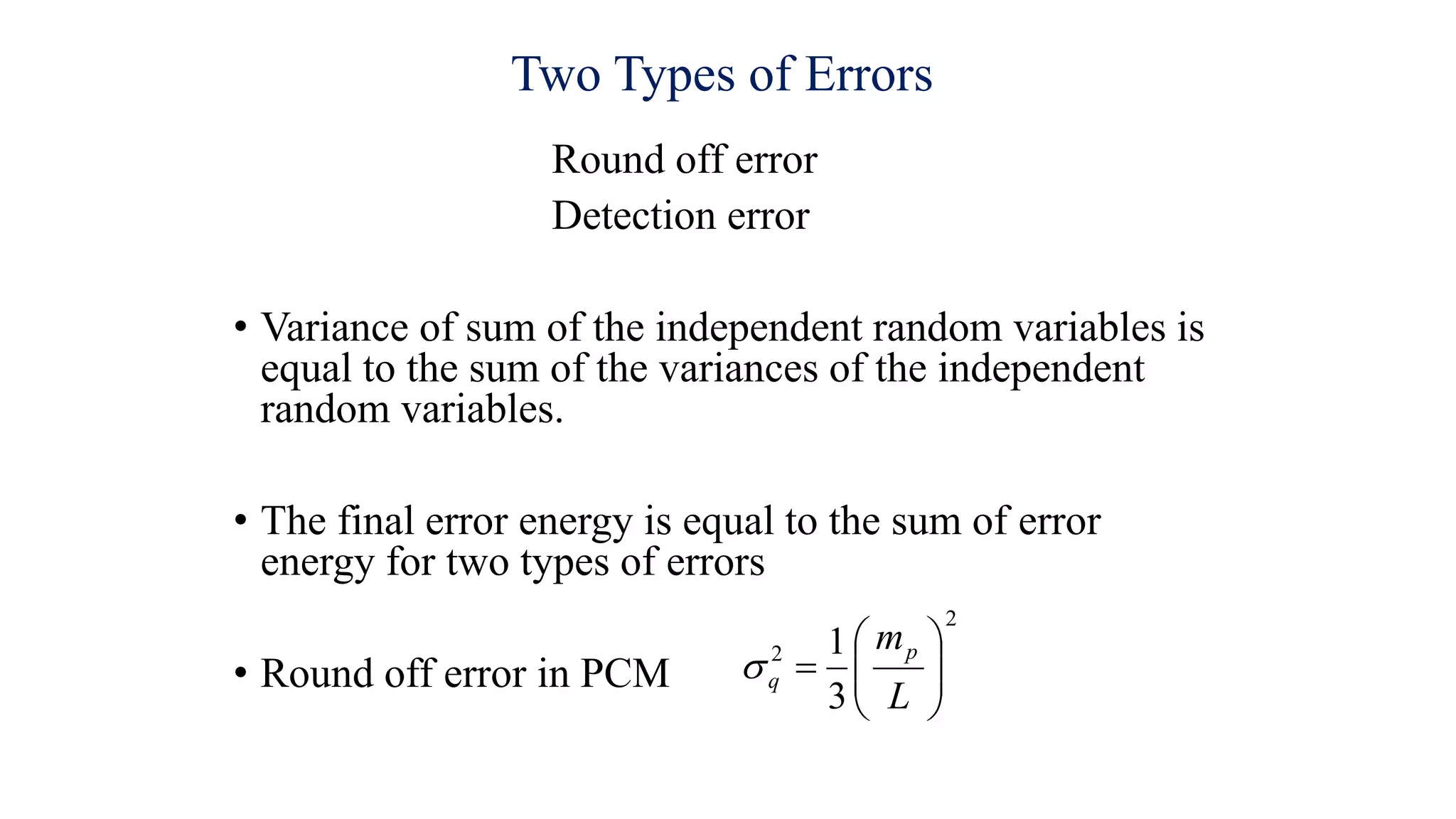
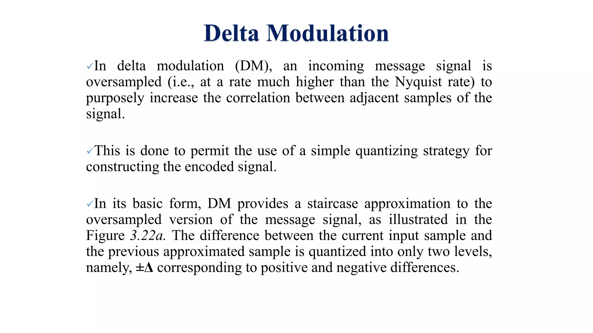
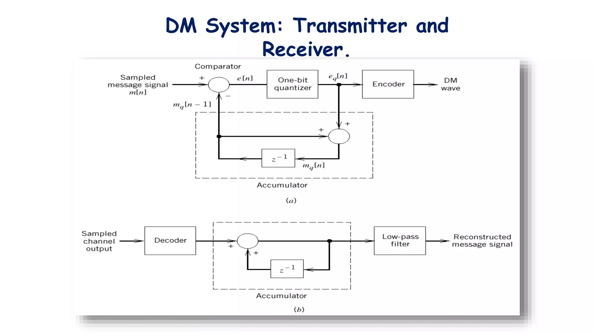
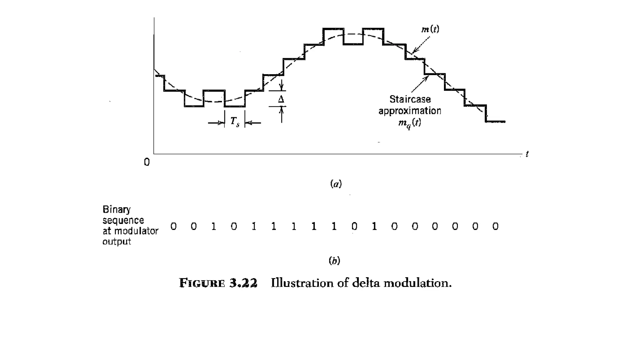
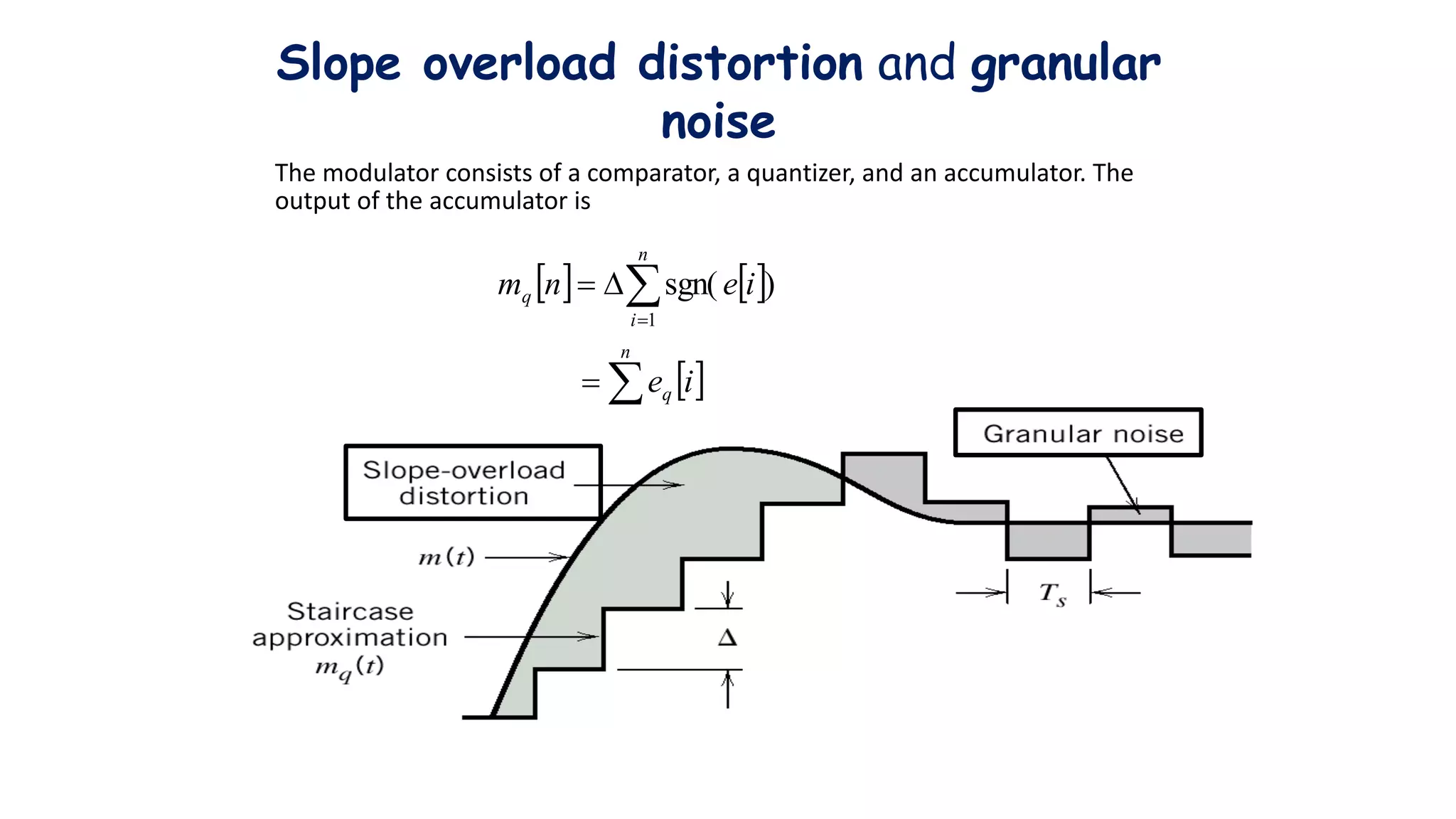
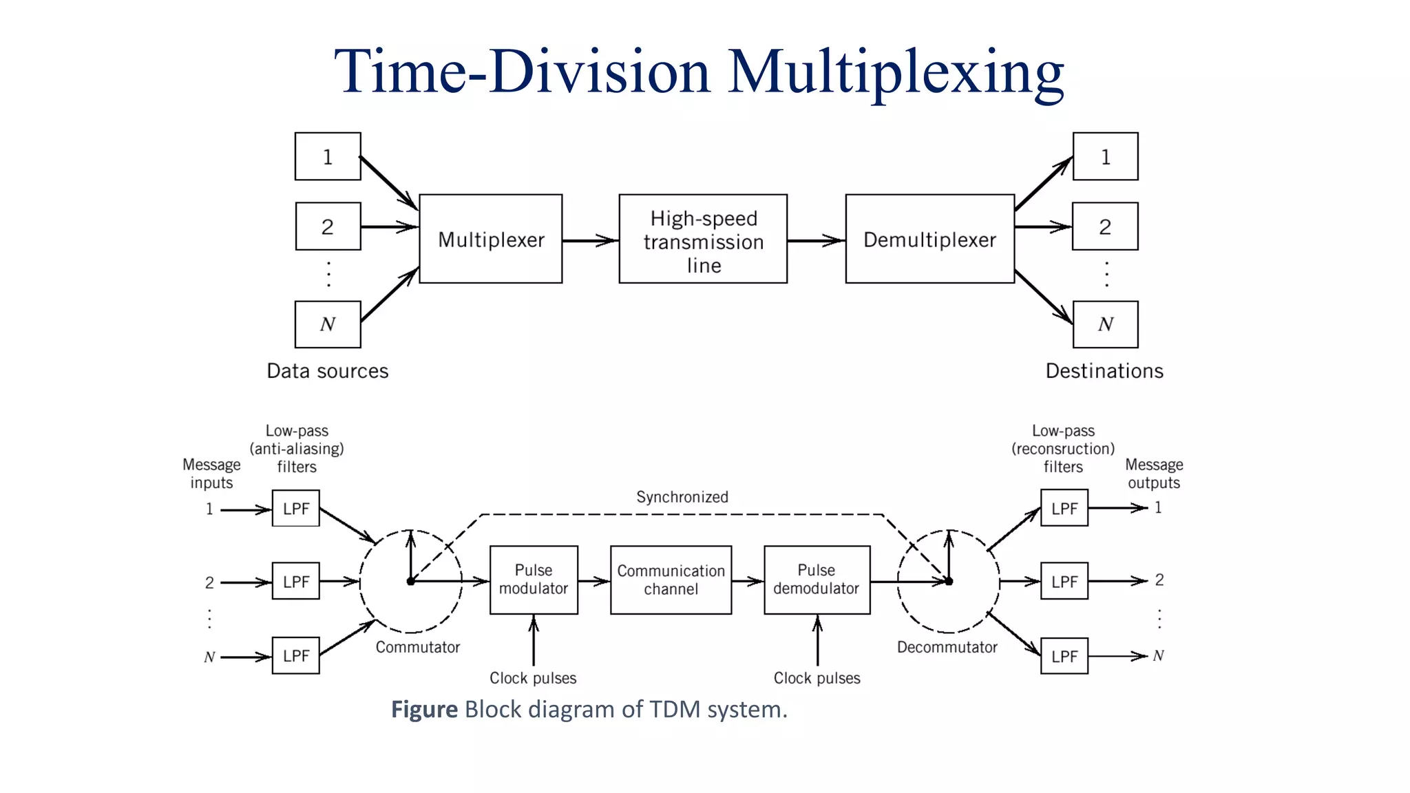
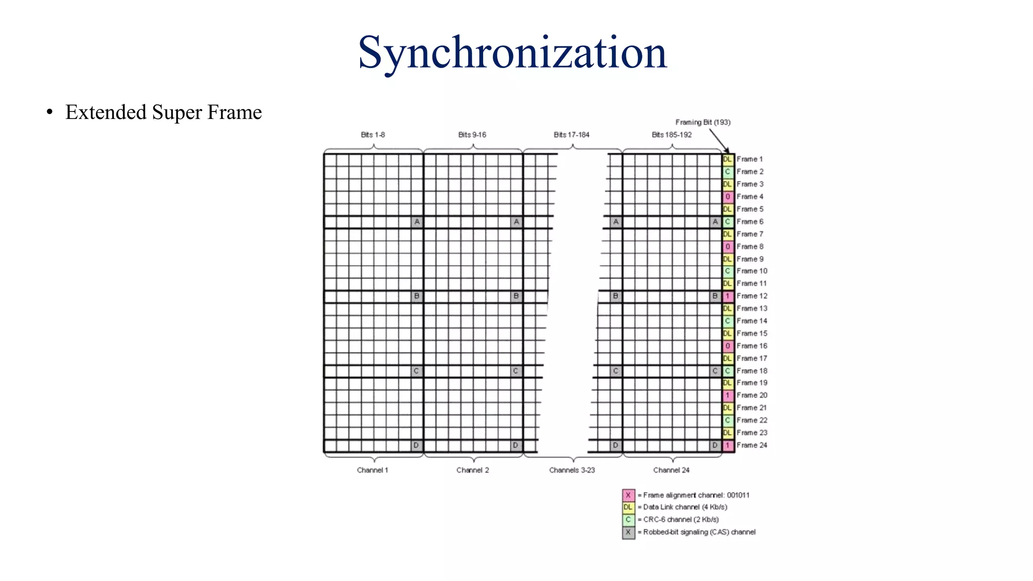
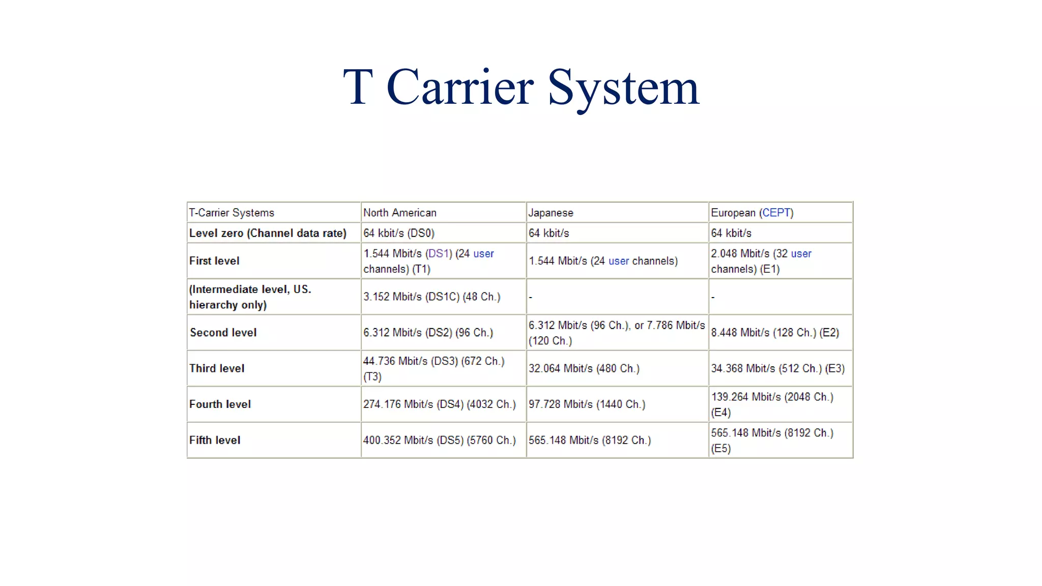
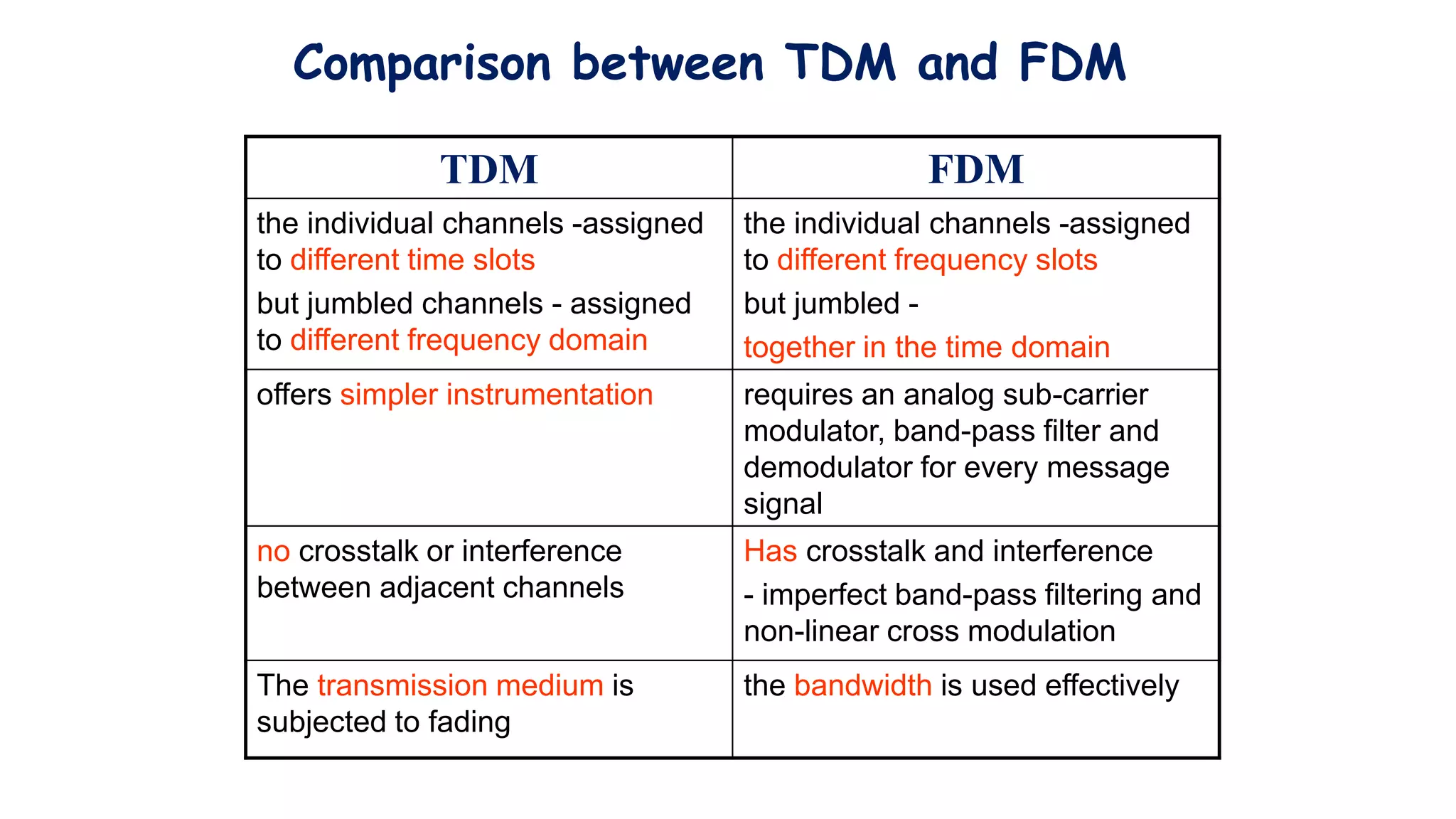
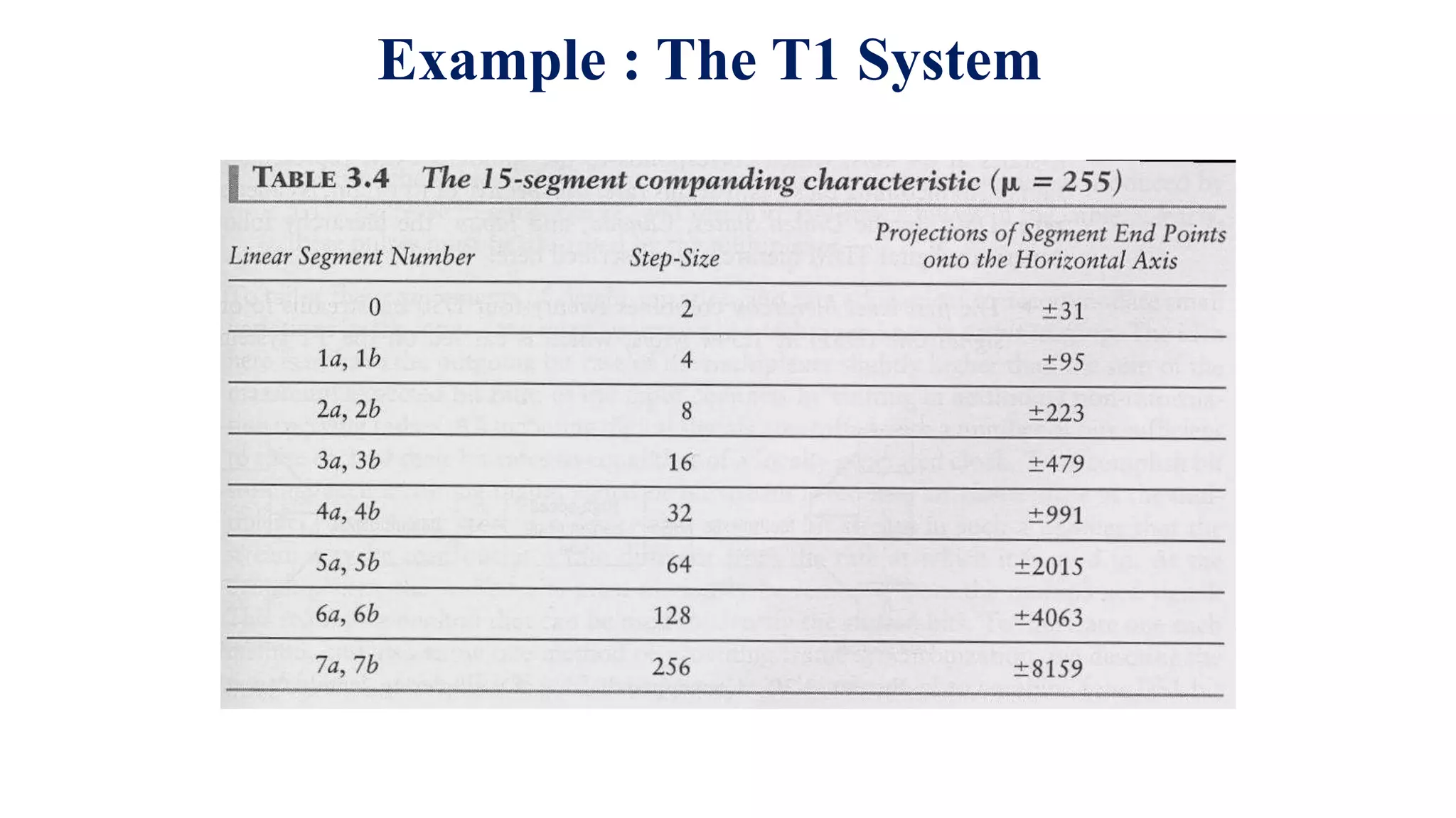
1. Prepared by
M.Paranthaman, AP/ECE
KNCET

2. Contents
• Sampling Process: Sampling Theorem
• Pulse Amplitude Modulation: Sample and Hold Filter
• Pulse Position Modulation
• Transition from Analog to Digital: Quantization process
• Pulse Code Modulation: Regeneration of signal in channel
• Delta Modulation: System details, Quantization Errors,
Delta/Sigma Modulation
• Differential Pulse Code Modulation
• Line codes
• Time Division Multiplexing: Synchronization
• Impulse Radio

5. Sampling
 Analog signal is sampled every TS secs.
 Ts is referred to as the sampling interval.
 fs = 1/Ts is called the sampling rate or sampling
frequency.
 There are 3 sampling methods:
– Ideal - an impulse at each sampling instant
– Natural - a pulse of short width with varying amplitude
– Flattop - sample and hold, like natural but with single
amplitude value
 The process is referred to as pulse amplitude
modulation PAM and the outcome is a signal with
analog (non integer) values

6. Figure :Three different sampling methods for PCM

7. Figure :Recovery of a sampled sine wave for different sampling rates

8. LP filter
Nyquist rate
aliasing

9. NYQUIST THEOREM
Nyquist theorem
• determine minimum sampling rate for any signal
• the signal will be correctly restored at the receiver
Nyquist’s Sampling Theorem states that;
The original information signal can be reconstructed at the receiver with minimal
distortion if the sampling rate in the pulse modulation system is equal to or
greater than twice the maximum information signal frequency.
• fs >= 2 fm(max)
• minimum sampling frequency; fs(min) = 2 fm(max)

10. NYQUIST RATE & NYQUIST INTERVAL
NYQUIST RATE
• Sampling rate becomes exactly equal to ‘2w’ samples/sec.
Nyquist rate= 2w Hz
NYQUIST INTERVAL
• Time interval between any two adjacent samples
Nyquist interval = 1/2w sec

11. Sample and Hold Circuit

12. Flat top PAM

13. Flat top PAM detection

14. PPM

16. PPM Detection

18. Shannon channel capacity
 Claude Shannon, a Bell Labs Mathematician,
proved in 1948 that a communication channel is
fundamentally speed-limited. This limit is given by
C=Wlog2(1+P/NoW) bits/sec
 Where W is channel’s bandwidth, P signal power
and No is noise spectral density

19. Quantization
 The output of a sampler is still continuous in amplitude.
◦ Each sample can take on any value e.g. 3.752, 0.001, etc.
◦ The number of possible values is infinite.
 To transmit as a digital signal we must restrict the number
of possible values.
 Quantization is the process of “rounding off” a sample
according to some rule.
◦ E.g. suppose we must round to the nearest tenth, then:
3.752 --> 3.8 0.001 --> 0

20. Uniform Quantization
 Most ADC’s use uniform quantizers.
 The quantization levels of a uniform quantizer are
equally spaced apart.
 Uniform quantizers are optimal when the input
distribution is uniform. When all values within the
Dynamic Range of the quantizer are equally likely.

21. Types of Quantizers:
1. Uniform Quantizer
2. Non- Uniform Quantizer
Uniform Quantizer: In Uniform type, the quantization levels are uniformly spaced,
whereas in non-uniform type the spacing between the levels will be unequal and
mostly the relation is logarithmic.
Types of Uniform Quantizers: ( based on I/P - O/P Characteristics)
1. Mid-Rise type Quantizer
2. Mid-Tread type Quantizer
In the stair case like graph, the origin lies the middle of the tread portion in Mid –Tread type
where as the origin lies in the middle of the rise portion in the Mid-Rise type.

24. Two types of quantization:
(a) midtread and (b) midrise.

25. Non – Uniform Quantizer:
In Non – Uniform Quantizer the step size varies. The use of a
non – uniform quantizer is equivalent to passing the baseband signal
through a compressor and then applying the compressed signal to a
uniform quantizer. The resultant signal is then transmitted.
COMPRESSOR UNIFORM QUANTIZER EXPANDER
At the receiver, a device with a characteristic complementary to the
compressor called Expander is used to restore the signal samples to
their correct relative level. The Compressor and expander take together
constitute a Compander.
Compander = Compressor + Expander

26. Quantization Example
Analogue signal
Sampling TIMING
Quantization levels.
Quantized to 5-levels
Quantization levels
Quantized 10-levels

27. Quantization
Noise
Figure Illustration of the quantization process. (Adapted from Bennett, 1948,
with permission of AT&T.)

30. Quantization (non-uniform
quantizer)

31. Figure Compression laws. (a) m -law. (b) A-law.

32. Pulse Code Modulation (PCM)
o Pulse code modulation (PCM) is produced by analog-to-digital conversion
process. Quantized PAM
• A uniform linear quantizer is called Pulse Code Modulation (PCM).
• Pulse code modulation (PCM): Encoding the quantized signals into a digital
word (PCM word or codeword).
• Each quantized sample is digitally encoded into an l bits codeword where
L in the number of quantization levels
o The sampling rate must be greater than, twice the highest frequency in the
analog signal,
fs > 2fA(max)
o Telegraph time-division multiplex (TDM) was conveyed as early as 1853, by
the American inventor M.B. Farmer. The electrical engineer W.M. Miner, in
1903.
o PCM was invented by the British engineer Alec Reeves in 1937 in France.
o It was not until about the middle of 1943 that the Bell Labs people became
aware of the use of PCM binary coding as already proposed by Alec Reeves.

33. OPERATION
 The PCM signal is generated by carrying out three basic
operations:
1. Sampling
2. Quantizing
3. Encoding
1. Sampling operation generates a flat-top PAM signal.
2. Quantizing operation approximates the analog values by
using a finite number of levels. This operation is considered
in 3 steps
a) Uniform Quantizer
b) Quantization Error
c) Quantized PAM signal output
3. PCM signal is obtained from the quantized PAM signal by
encoding each quantized sample value into a digital word.

34. Analog to Digital Conversion
 The Analog-to-digital Converter (ADC)
performs three functions:
◦ Sampling
 Makes the signal discrete in time.
 If the analog input has a bandwidth of
W Hz, then the minimum sample
frequency such that the signal can be
reconstructed without distortion.
◦ Quantization
 Makes the signal discrete in amplitude.
 Round off to one of q discrete levels.
◦ Encode
 Maps the quantized values to digital
words that are  bits long.
 If the (Nyquist) Sampling Theorem is
satisfied, then only quantization introduces
distortion to the system.
ADC
Sample
Quantize
Analog
Input
Signal
Encode
111
110
101
100
011
010
001
000
Digital Output
Signal
111 111 001 010 011 111 011

35. Figure The basic elements of a PCM system.
Pulse Code Modulation

36. 0000
1111
1110
1101
1100
1011
1010
1001
0001
0010
0011
0100
0101
0110
0111
0000 0110 0111 0011 1100 1001 1011
Numbers passed from ADC to computer to represent analogue voltage
Resolution=
1 part in 2n
PCM

37. pwm
ppm
pam
pcm
Analog pulse
modulation
Digital PM
-Converted into pulses by the process of sampling

38. Encoding
• The output of the quantizer is one of M possible signal levels.
• If we want to use a binary transmission system, then we need to map
each quantized sample into an n bit binary word.
• Encoding is the process of representing each quantized sample by an  bit
code word.
• The mapping is one-to-one so there is no distortion introduced by
encoding.
• There are many ways of doing this
• Natural coding
• Gray coding
• Some mappings are better than others.
• A Gray code gives the best end-to-end performance.
• The weakness of Gray codes is poor performance when the sign bit
(MSB) is received in error.
2
2 , log ( )
n
M n M
 

39. Encoding

40. Virtues, Limitations and Modifications of
PCM:
Advantages of PCM
1. Robustness to noise and interference
2. Efficient regeneration
3. Efficient SNR and bandwidth trade-off
4. Uniform format
5. Ease add and drop
6. Secure
Disadvantages of PCM
1. It requires large bandwidth
2. System complexity also increased
Modifications of PCM
1.VLSI chips are made commercially available for PCM system
2. Increased bandwidth is provided by OFC optical fibre cable
3 Using data compression techniques ,redundancy and transmitted data bit rate is reduced
4. Instead of PCM, Delta modulation also preffered

41. Noise consideration in PCM systems
(Channel noise, quantization noise)

42. Noise consideration in PCM system
The performance of a PCM system is influenced by two major
sources of noise.
1) Channel noise, which is introduced anywhere between the
transmitter output and the receiver input, channel noise is always
present, once the equipment is switched on.
2) Quantization noise, which is introduced in the
transmitter and is carried all the way along to the receiver
output.

43. Two Types of Errors
Round off error
Detection error
• Variance of sum of the independent random variables is
equal to the sum of the variances of the independent
random variables.
• The final error energy is equal to the sum of error
energy for two types of errors
• Round off error in PCM
2
2
3
1









L
mp
q


44. 1. Unipolar nonreturn-to-zero (NRZ) Signaling
2. Polar nonreturn-to-zero(NRZ) Signaling
3. Unipolar nonreturn-to-zero (RZ) Signaling
4. Bipolar nonreturn-to-zero (BRZ) Signaling
5. Split-phase (Manchester code)
Line codes

45. Figure Line codes for the electrical representations of binary data.
(a) Unipolar NRZ signaling. (b) Polar NRZ signaling.
(c) Unipolar RZ signaling. (d) Bipolar RZ signaling.
(e) Split-phase or Manchester code.

46. Differential Encoding
(encode information in terms of signal
transition; a transition is used to designate Symbol 0)
Regeneration (reamplification, retiming, reshaping )
Two measure factors: bit error rate (BER) and jitter.

48. Delta Modulation
In delta modulation (DM), an incoming message signal is
oversampled (i.e., at a rate much higher than the Nyquist rate) to
purposely increase the correlation between adjacent samples of the
signal.
This is done to permit the use of a simple quantizing strategy for
constructing the encoded signal.
In its basic form, DM provides a staircase approximation to the
oversampled version of the message signal, as illustrated in the
Figure 3.22a. The difference between the current input sample and
the previous approximated sample is quantized into only two levels,
namely, ±Δ corresponding to positive and negative differences.

49. DM System: Transmitter and
Receiver.

51. The modulator consists of a comparator, a quantizer, and an accumulator. The
output of the accumulator is
   
 
)
sgn(
1
1







n
i
q
n
i
q
i
e
i
e
n
m
Slope overload distortion and granular
noise

52.  
     
   
     
   
  size
step
the
is
and
,
of
version
quantized
the
is
,
output
quantizer
the
is
where
1
)
sgn(
1
is
signal
error
The
).
(
of
sample
a
is
)
(
and
period
sampling
the
is
where
,
2
,
1
,
0
,
)
(
Let













n
e
n
e
n
m
n
e
n
m
n
m
n
e
n
e
n
m
n
m
n
e
t
m
nT
m
T
n
nT
m
n
m
q
q
q
q
q
q
q
s
s
s 

53. The modulation which has an integrator can
relieve the draw back of delta modulation (differentiator)
Beneficial effects of using integrator:
1. Pre-emphasize the low-frequency content
2. Increase correlation between adjacent samples
(reduce the variance of the error signal at the quantizer
input )
3. Simplify receiver design
Because the transmitter has an integrator , the receiver
consists simply of a low-pass filter.
(The differentiator in the conventional DM receiver is
cancelled by the integrator )



Delta-Sigma modulation (sigma-delta modulation)

54. delta-sigma modulation system.

55. Differential Pulse-Code Modulation (DPCM)
Usually PCM has the sampling rate higher than the Nyquist rate.
The encode signal contains redundant information. DPCM can efficiently remove
this redundancy.

56. MULTIPLEXING
Multiplexing is a technique of more than one source to more
than one destination on the same medium.
There are two common techniques of multiplexing:
FDMA(frequency division multiple access)
 TDMA(time division multiple access)
CDMA(code division multiple access)

57. FDMA
 In FDM, multiple users can be on at the same time
by placing them in orthogonal frequency bands
guardband
user 1 user 2 user N
TOTAL BANDWIDTH

58. Digital
Multiplexers

59. Basic idea behind TDMA
 Take the following 3 digital lines
frame

60. Time-Division Multiplexing
Figure Block diagram of TDM system.

61. DS1/E1/T1
• Digital signal 1 (DS1, also known as T1) is a T-carrier signaling
scheme devised by Bell Labs. DS1 is a widely used standard in
telecommunications in North America and Japan to transmit voice and data
between devices. E1 is used in place of T1 outside of North America and
Japan. Technically, DS1 is the transmission protocol used over a physical T1
line; however, the terms "DS1" and "T1" are often used interchangeably.
• A DS1 circuit is made up of twenty-four DS0
• DS1: (8 bits/channel * 24 channels/frame + 1 framing bit) * 8000 frames/s =
1.544 Mbit/s
• A E1 is made up of 32 DS0
• The line data rate is 2.048 Mbit/s which is split into 32 time slots, each being

62. T1 bit rate per frame
•Data rate
•8x24=192 bits per frame
•Framing bit rate
•1 bit per frame
•Total per frame
•193 bits/frame
©2000 Bijan Mobasseri

63. Total T1 bit rate
•We know there are 8000 frames a sec. and there
are 193 bits per frame. Therefore
T1 rate=193x8000=1.544 Mb/sec

64. Signaling rate component
•Not all 1.544 Mb/sec is data. In every 6th frame,
we replace 24 data bits by signaling bits.
Therefore
signaling rate= (8000frames/sec)(1/6)(24 bits)=32
Kbits/sec

65. Synchronization

66. Synchronization
• Extended Super Frame

67. T Carrier System

68. TDM FDM
the individual channels -assigned
to different time slots
but jumbled channels - assigned
to different frequency domain
the individual channels -assigned
to different frequency slots
but jumbled -
together in the time domain
offers simpler instrumentation requires an analog sub-carrier
modulator, band-pass filter and
demodulator for every message
signal
no crosstalk or interference
between adjacent channels
Has crosstalk and interference
- imperfect band-pass filtering and
non-linear cross modulation
The transmission medium is
subjected to fading
the bandwidth is used effectively
Comparison between TDM and FDM

69. Example : The T1 System