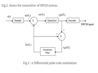
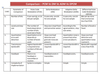
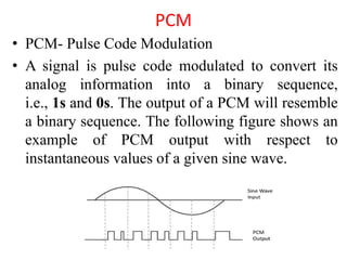
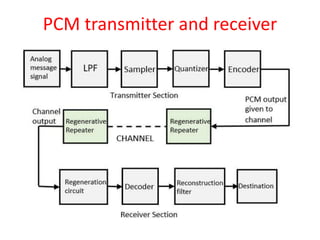
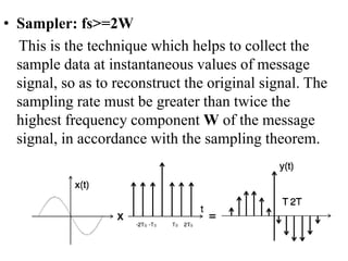
This document provides an overview of several waveform coding and representation techniques, including PCM, DM, ADM, and DPCM. PCM converts an analog signal into a digital binary sequence by sampling, quantizing, and encoding the signal. DM and ADM transmit only one bit per sample and adapt the step size used for quantization. DPCM uses prediction to transmit only the difference between the predicted and actual signal values, requiring fewer bits.

1. UNIT 2 WAVEFORM CODING AND
REPRESENTATION
• DM
• DPCM
• LPC
• LINE CODES

2. PCM
• PCM- Pulse Code Modulation
• A signal is pulse code modulated to convert its
analog information into a binary sequence,
i.e., 1s and 0s. The output of a PCM will resemble
a binary sequence. The following figure shows an
example of PCM output with respect to
instantaneous values of a given sine wave.

3. • PCM produces a series of numbers or digits, and
hence this process is called as digital. Each one of
these digits, though in binary code, represent the
approximate amplitude of the signal sample at that
instant.
• In Pulse Code Modulation, the message signal is
represented by a sequence of coded pulses. This
message signal is achieved by representing the signal
in discrete form in both time and amplitude.

4. PCM transmitter and receiver

5. • Sampler: fs>=2W
This is the technique which helps to collect the
sample data at instantaneous values of message
signal, so as to reconstruct the original signal. The
sampling rate must be greater than twice the
highest frequency component W of the message
signal, in accordance with the sampling theorem.

6. • Quantizer is a process of reducing the excessive
bits and confining the data. The sampled output
when given to Quantizer, reduces the redundant
bits and compresses the value.

7. • Encoder
The digitization of analog signal is done by the
encoder. It designates each quantized level by a
binary code. The sampling done here is the sample-
and-hold process. These three sections
LPF,Sampler,and Quantizer will act as an analog to
digital converter. Encoding minimizes the bandwidth
used.
SIGNAL  BINARY DIGITS

8. ADVANTAGES
• The PCM (pulse code modulation) convenient
for long distance communication.
• It has a higher transmitter efficiency.
• It has a higher noise immunity.

9. DISADVANTAGES
• The PCM (pulse code modulation) requires
large bandwidth as compared to analog
system.
• Encoding, decoding and quantizing circuit of
PCM is very complex.

10. DELTA MODULATION AND
ADAPTIVE DELTA
MODULATION

11. DM-Principle
• It transmits only one bit per sample.
• The present sample value is compared with previous sample
value.The input signal x(t) is approximated to step signal by
delta modulator.
• The difference betweeninput signal and staircase approximated
signal confined to two levels + δ and - δ .
• If the difference is positive then approximated signal is
increased by one step i.e ‘δ’ and ‘1’ is transmitted.
• If the difference is negative then approximated signal is
reduced by i.e ‘δ’ and ‘0’ is transmitted.

12. Delta Modulation
• The type of modulation, where the sampling
rate is much higher and in which the stepsize
after quantization is of a smaller value Δ, such
a modulation is termed as delta modulation.
• Delta Modulation is a simplified form of
DPCM technique, also viewed as 1-bit DPCM
scheme. As the sampling interval is reduced,
the signal correlation will be higher.

13. Following are some of the features of delta modulation.
• An over-sampled input is taken to make full use of the signal
correlation.
• The quantization design is simple.
• The input sequence is much higher than the Nyquist rate.
• The quality is moderate.
• The design of the modulator and the demodulator is simple.
• The stair-case approximation of output waveform.
• The step-size is very small, i.e., Δ delta.
• The bit rate can be decided by the user.
• This involves simpler implementation.

14. DM Transmitter

15. BLOCK DIAGRAM EXPLANATION
• The predictor circuit in DPCM is replaced by a
simple delay circuit in DM.
• From the above diagram, we have the notations
as
• x(nTs) = over sampled input/input signal
• ep(nTs) = summer output and quantizer input
• eq(nTs) = quantizer output = v(nTs)v(nTs)
• xˆ(nTs) = output of delay circuit/reconstructed
signal
• u(nTs) = input of delay circuit

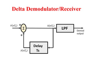
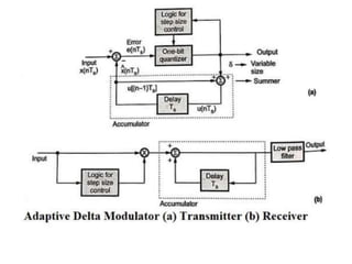
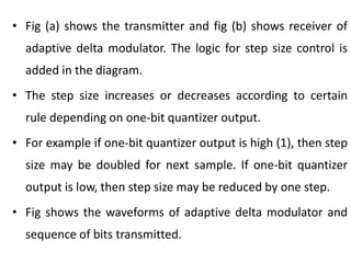
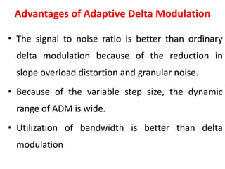
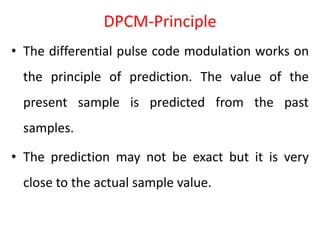
16. • x^(nTs) = the previous value of the delay circuit
• eq(nTs) = quantizer output = v(nTs)
• Hence,
• u(nTs)=u([n−1]Ts)+v(nTs)
x^(nTs) = u([n−1]Ts)
CONDITION:
x(nTs) > x^(nTs) = + δ = 1
x(nTs) < x^(nTs) = - δ = 0
Accumulator is used to provide latest reconstructed signal

17. Delta Demodulator/Receiver

18. DM receiver
• The DM signal is added with one bit delayed
reconstructed signal. This is accumulator operation
• The reconstructed signal is then passed through low
pass filter for smoothing.
• If the input signal is binary “1” then it adds + δ to the
previous output. If the input signal is binary “0” then
one step δ is subtracted from the delayed signal.
• Maximum quantization error in DM is εmax = IδI

19. Advantages of DM Over DPCM
• 1-bit quantizer
• Very easy design of the modulator and the
demodulator
However, there exists some noise in DM.
• Slope Over load distortion (when Δ is small)
• Granular noise (when Δ is large)

20. DRAWBACKS
• Slope overload distortion arises because of large dynamic
range of the input signal or in other words under
maximum slope of the signal or the rate of rise of input
signal x(t) is so high, step size becomes small to follow the
step of the input waveform. This condition is called slope
overload and the resulting quantization error is called slope
overload distortion.
• Granular noise is the manifestation of random signals when
the variation of the input signal is smaller than the step size.
It occurs when the step size is too large compared to small
variations in input signal.

21. DM OUTPUT

22. ADM
• In digital modulation, we have come across certain problem of
determining the step-size, which influences the quality of the
output wave.
• A larger step-size is needed in the steep slope of modulating
signal and a smaller stepsize is needed where the message has a
small slope. The minute details get missed in the process. So, it
would be better if we can control the adjustment of step-size,
according to our requirement in order to obtain the sampling in
a desired fashion. This is the concept of Adaptive Delta
Modulation.

23. ADM
• To overcome the quantization errors due to
slope overload and granular noise, the step size
(δ) is made adaptive to variations in the input
signal x(t). Particularly in the steep segment of
the signal x(t), the step size is increased. When
the input is varying slowly, the step size is
reduced. Then the method is called Adaptive
Delta Modulation (ADM).

25. • Fig (a) shows the transmitter and fig (b) shows receiver of
adaptive delta modulator. The logic for step size control is
added in the diagram.
• The step size increases or decreases according to certain
rule depending on one-bit quantizer output.
• For example if one-bit quantizer output is high (1), then step
size may be doubled for next sample. If one-bit quantizer
output is low, then step size may be reduced by one step.
• Fig shows the waveforms of adaptive delta modulator and
sequence of bits transmitted.

26. • In the receiver of adaptive delta modulator shown in Fig
(b) the first part generates the step size from each
incoming bit.
• Exactly the same process is followed as that in transmitter.
The previous input and present input decides the step
size.
• It is then given to an accumulator which builds up
staircase waveform. The low-pass filter then smoothens
out the staircase waveform to reconstruct the smooth

27. ADM OUTPUT

28. Continuously variable slope delta
modulation (CVSD)
• In ADM, the step size changes in discrete
steps.
• When the step size varies continuously, then it
is called continuously variable slope delta
modulation (CVSD).

29. Advantages of Adaptive Delta Modulation
• The signal to noise ratio is better than ordinary
delta modulation because of the reduction in
slope overload distortion and granular noise.
• Because of the variable step size, the dynamic
range of ADM is wide.
• Utilization of bandwidth is better than delta
modulation

30. DPCM-Principle
• The differential pulse code modulation works on
the principle of prediction. The value of the
present sample is predicted from the past
samples.
• The prediction may not be exact but it is very
close to the actual sample value.

32. • The sampled signal is denoted by x(nTs) and predicted
signal is denoted by xˆ(nTs).
• The comparator finds out the difference between the
actual sample value x(nTs) and predicted sample value
xˆ(nTs).
• This is known as prediction error and it is denoted by
e(nTs).
• It can be defined as ,
• e(nTs) = x(nTs) – xˆ(nTs)……………………….(1)
• The predicted value is produced by using a prediction filter.

33. • The quantizer output signal gap eq(nTs) and previous prediction is
added and given as input to the prediction filter.This signal is
called xq(nTs).
• This makes the prediction more and more close to the actual sampled
signal.We can observe that the quantized error signal eq(nTs) is very
small and can be encoded by using small number of bits.
• Thus number of bits per sample are reduced in DPCM.
• The quantizer output can be written as ,
• eq(nTs) = e(nTs) + q(nTs)………………………..(2)
• Here, q(nTs) is the quantization error.

34. • As shown in fig.2, the prediction filter input xq(nTs) is
obtained by sum xˆ(nTs) and quantizer output. i.e.,
• xq(nTs) = xˆ(nTs) + eq(nTs)……………………..(3)
• Substituting the value of eq(nTs) from eq.(2) in the
above eq. (3) , we get,
• xq(nTs) = xˆ(nTs) + e(nTs) + q(nTs) ………………….(4)
• eq.(1) is written as,
• e(nTs) = x(nTs) – xˆ(nTs)
• e(nTs) + xˆ(nTs) = x(nTs)
• Therefore, substituing the value of e(nTs) + xˆ(nTs)
from the above equation into eq. (4), we get,
• xq(nTs) = x(nTs) + q(nTs) …………………..(5)

36. • The decoder first reconstructs the quantized
error signal from incoming binary signal.
• The prediction filter output and quantized error
signals are summed up to give the quantized
version of the original signal.
• Thus the signal at the receiver differs from actual
signal by quantization error q(nTs), which is
introduced permanently in the reconstructed
signal.

37. Advantages of DPCM
• As the difference between x(nTs) and xˆ(nTs) is being
encoded and transmitted by the DPCM technique, a
small difference voltage is to be quantized and
encoded.
• This will require less number of quantization levels
and hence less number of bits to represent them.
• Thus signaling rate and bandwidth of a
DPCM system will be less than that of PCM.

38. LINEAR PREDICTIVE CODING
• LPC is a tool which represents digital speech signals in
linear predictive model.
• This is mostly used in audio signal processing, speech
synthesis, speech recognition, etc.
• Linear prediction is based on the idea that the current
sample is based on the linear combination of past
samples.
• The analysis estimates the values of a discrete-time signal
as a linear function of the previous samples.

39. Speech model used in voice coders

40. • There are two frequency sources
• One frequency source is used to generate unvoiced
sound. Such sound are generated when the speaker
pronounces letter such as s,f. A noise source is used
to generate such unvoiced sounds.
• The voice sound are simulaed by impulse
generator.The frequency of this generator is varied
depending upon the pitch of the sound.
• These voiced or unvoiced passes through the filter.
This filter represent vocal tract.
• In vocal tract this operation is done with the help of
tongue,teeth,lips etc.

41. LPC Transmitter

42. LPC Transmitter
• The analyzer determines LP coefficients for the synthesis
filter.
• Based on the LP coefficient the synthesis filter
reconstruct the speech signal.
• The reconstructed signal and the original signal are
compared and error is obtained.
• The LP coefficients and the error signal is multiplexed
and transmitted.This signal is called LPC signal

43. LPC RECEIVER

44. • The received LPC signal is applied to
demultiplexer or decoder.It seperates filter
parameters and error signal.
• The LP coefficients are given to the synthesis
filter.
• The output of synthesis filter is added to error
signal which gives speech signal .
• The analyzer is a digital filter.

45. Comparison – PCM Vs DM Vs ADM Vs DPCM

46. Line Coding
Properties:
1) Less transmission bandwidth
2) Less Power Efficiency
3) Easy error detection and
correction
4) Power Spectral Density
5) Adequate timing content
6) Transparency

47. Properties of line coding
• As the coding is done to make more bits transmit on
a single signal, the bandwidth used is much reduced.
• For a given bandwidth, the power is efficiently used.
• The probability of error is much reduced.
• Error detection is done and the bipolar too has a
correction capability.
• Power density is much favorable.
• The timing content is adequate.
• Long strings of 1s and 0s is avoided to maintain
transparency.

48. TYPES
There are 3 types of Line Coding
• Unipolar
• Polar
• Bi-polar
SIGNAL Representation
• NRZ- Not Return to ZERO
• RZ – Return to ZERO

53. UNIPOLAR NRZ

54. UNIPOLAR RZ

55. POLAR NRZ

56. POLAR RZ

57. BIPOLAR NRZ & RZ