Statistics 522: Sampling and Survey Techniques
                                        Topic 6

Topic Overview
This topic will cover

   • Sampling with unequal probabilities

   • Sampling one primary sampling unit

   • One-stage sampling with replacement


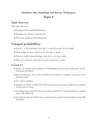
Unequal probabilities
   • Recall πi is the probability that unit i is selected as part of the sample.

   • Most designs we have studied so far have the πi equal.

   • Now we consider general designs where the πi can vary with i.

   • There are situations where this can give much better results.

Example 6.1
   • Survey of nursing home residents in Philadelphia to determine preferences on life-
     sustaining treatments

   • 294 nursing homes with a total of 37,652 beds (number of residents not known at the
     planning stage)

   • Use cluster sampling

   • Suppose we choose an SRS of the 294 nursing homes and then an SRS of 10 residents
     of each selected home.

   • A nursing home with 20 beds has the same probability of being sampled as a nursing
     home with 1000 beds.

   • 10 residents from the 20 bed home represent fewer people than 10 residents from 1000
     bed home.


                                              1
Self-weighting
   • This procedure gives a sample that is not self-weighted.

   • Alternatives that are self-weighted.

       – A one-stage cluster sample
       – Sample a fixed percentage of the residents of each selected nursing home.

The two-stage cluster design
   • The two-stage cluster design (SRS of homes, then equal proportion SRS of residents
     in each selected home)

       – Gives a mathematically valid estimator

SRS at first stage
Three shortcomings:

   • We would expect ti to be proportional to the number of beds in nursing home i, so
     estimators will have large variance (Mi ).

   • Equal percentage sampling in each selected home may be difficult to administer.

   • Cost is not known in advance (dont know if you will get large or small homes in sample).

The study
   • They drew a sample of 57 nursing homes with probabilities proportional to the number
     of beds.

   • Then they took an SRS of 30 beds (and their occupants) from a list of all beds within
     each selected nursing home.

Properties
   • Each bed is equally likely to be in the sample (note beds vs occupants).

   • The cost is known before selecting the sample.

   • The same number of interviews is taken at each nursing home.

   • The estimators will have smaller variance


                                             2
Key ideas
  • When sampling with unequal probabilities, we deliberately vary the selection proba-
    bilities.

  • We compensate by using weights in the estimation.

  • The key is that we know the selection probabilities

Notation
  • The probability that psu i is in the sample is πi .

  • The probability that psu i is selected on the first draw is ψi .

  • We will consider an artificial situation where n = 1, so πi = ψi .

Sampling one psu
  • Sample size is n = 1.

  • Suppose we are interested in estimating the population total.

  • ti is the total for psu i.

  • To illustrate the ideas, we will assume that we know the whole population.


The Example
  • N = 4 supermarkets

  • Size (in square meters) varies.

  • Select n = 1 with probabilities proportional to size.

  • Record total sales

  • Using the data from one store we want to estimate total sales for the four stores in the
    population.

The population
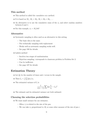
                                 Store    Size          ψi   ti
                                   A      100         1/16 11
                                   B      200         2/16 20
                                   C      300         3/16 24
                                   D     1000        10/16 245
                                 Total   1600            1 300

                                                 3
Weights
   • The weights wi are the inverses of the selection probabilities ψi .

   • The weighted estimator of the population total is tψ =
                                                       ˆ             wi ti .

   • There are four possible samples.

   • We calculate tψ for each.
                  ˆ


The samples
                              Sample    ψi        wi         ti ˆ
                                                                tψ
                                A     1/16        16        11 176
                                B     2/16         8        20 160
                                C     3/16      16/3        24 128
                                D    10/16     16/10       245 392

                                      ˆ
Sampling distribution of the estimate tψ
                                    Sample    ψi        ˆ
                                                        tψ
                                      1     1/16       176
                                      2     2/16       160
                                      3     3/16       128
                                      4    10/16       392

                                     ˆ
Mean of the sampling distribution of tψ

                     ˆ      1       2     3     10
                   E tψ =      176 + 160 + 128 + 392 = 300 = t
                            16      16    16    16
   • So tψ is unbiased.
        ˆ

   • This will always be true.

                                     ˆ
                                   E tψ =     ψi wi ti =     ti

                                      ˆ
Variance of the sampling distribution tψ

             1                2              3              10
    ˆ
Var(tψ ) =      (176 − 300)2 + (160 − 300)2 + (128 − 300)2 + (392 − 300)2 = 14248
             16               16             16             16
Compare with the variance for an SRS:
            1              1              1              1
Var(tSRS ) = (176 − 300)2 + (160 − 300)2 + (128 − 300)2 + (392 − 300)2 = 154488
    ˆ
            4              4              4              4

                                              4
Interpretation
  • Store D is the largest and we expect it to account for a large portion of the total sales.

  • Therefore, we give it a higher probability of being in the sample (10/16) than it would
    have with an SRS (1/4).

  • If it is selected, we multiply its sales by (16/10) to estimate total sales.


One-stage sampling with replacement
  • Suppose n > 1 and we sample with replacement.

  • This implies πi = 1 − (1 − ψi )n .

  • Probability that item i is selected on the first draw is the same as the probability that
    item i is selected on any other draw.

  • Sampling with replacement gives us n independent estimates of the population total,
    one for each unit in sample.

  • We average these n estimates.

  • Estimated variance is variance of the estimates divided by n

Example 6.2
  • N = 15 classes of elementary stat

  • Mi students in class i (i = 1 to 15)

  • Values of Mi range from 20 to 100.

  • We want a sample of 5 classes.

  • Each student in the selected classes will fill out a questionnaire.

  • (It is possible for the same class to be selected more than once.)

Randomization
  • There are a total of 647 students in these classes.

  • Select 5 random numbers between 1 and 647.

  • Think about ordering the students by class.

  • Each random number corresponds to a student and the corresponding class will be in
    the sample.

                                              5
This method
  • This method is called the cumulative-size method.
  • It is based on M1 , M1 + M2 , M1 + M2 + M3 , . . .
  • An alternative is to use the cumulative sums of the ψi and select random numbers
    between 0 and 1.
  • For this example, ψi = Mi /647

Alternative
  • Systematic sampling is often used as an alternative in this setting.
       – The basic idea is the same.
       – Not technically sampling with replacement
       – Works well as systematic sampling works well.
       – See page 186 for details.
  • Lahiris method
       – Involves two stages of randomization
       – Rejection sampling: corresponds to classroom problem in Problem Set 2.
       – Can be inefficient.
       – See page 187 for details


Estimation Theory
  • Let Qi be the number of times unit i occurs in the sample.
                1
  • Then tψ =
         ˆ
                n
                     Qi ti /ψi .

  • The estimated variance of ti is
                              ˆ
                                      1                  ti
                                                  Qi (      − tψ )2
                                                              ˆ
                                   n(n − 1)              ψi

  • The estimate and its estimated variance are both unbiased.

Choosing the selection probabilities
  • We want small variance for our estimator.
       – Often, ti is related to the size of the psu.
       – We can take ψi proportional to Mi or some other measure of the size of psu i.

                                              6
PPS
  • This procedure is called sampling with probability proportional to size (pps).

  • The formulas for the estimate and variance can be simplified for this special case.
                                                   Mi
                                          ψi =
                                                   K
                                          ti
                                             = K yi
                                                 ¯
                                          ψi

  • See page 190 for details

  • See Example 6.5 on pages 190-192

Two-stage sampling with replacement
  • Basic ideas are very similar to one-stage sampling.

  • ψi is the probability that psu i is selected on the first (or any) draw.

  • We take a sample of mi ssus from each selected psu.

Sampling ssu’s
  • Usually we use an SRS.

  • Alternatives include

       – systematic sampling
       – any other probability sampling method

  • Note if a psu is selected more than once, a separate independent second stage sample
    is required.

Estimates and SE’s
  • Weights are used to make the estimators unbiased.

  • Formulas are similar to those for one-stage.

  • See (6.8) and (6.9) on page 192


                                            7
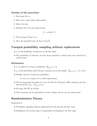
Outline of the procedure
  1. Determine the ψi .

  2. Select the n psus (with replacement).

  3. Select the ssus.

  4. Estimate the t for each selected psu,

                                        tψ = weight × t
                                        ˆ             ˆ

                             ˆ
  5. The average of these is tψ .
                                           √
  6. SE is the standard error of these (sd/ n).


Unequal probability sampling without replacement
   • ψi is the probability of selection on the first draw.

   • The probability of selection on later draws depends on which units were selected on
     earlier draws.

Estimation
   • πi is called the inclusion probability. (   pop   πi = n)

   • πi,j is the probability that both psu i and psu j are in the sample. (   j=i   πi,j = (n−1)πi )

   • Weights (inverse of selection probability)

        – we use πi /n in place of ψi (with replacement)

   • The recommended procedure is to use the Horvitz-Thompson (HT) estimator and the
                     ˆ         ˆ
     associated SE. (tHT = sam ti /πi )

   • See page 196-197 for details.

   • This estimator can be generalized to other designs that do not use replacement.


Randomization Theory
Framework is

   • Probability sampling without replacement for the psus for the first stage

   • Sampling at the second stage is independent of sampling at the first stage


                                                 8
Horvitz-Thompson
  • Randomization theory can be used to prove the Horvitz-Thompson Theorem.

      – Expected value of the estimator is t.
      – Formula for the variance of the estimator

The estimator
  • tHT =
    ˆ         ˆ
              ti /πi

      – where the sum is over the psu’s selected in the first stage.

  • Idea behind proofs is to condition on which psus are in the sample.

  • Study pages 205-210


Model
  • One-way random effects anova model

                                           Yi,j = Ai +   i,j


    where
                                                              2
      – the Ai are random variables with mean µ and variance σA
      – the   i,j   are random variables with mean 0 and variance σ 2 .
      – the Ai and the      i,j   are uncorrelated

The pps estimator
  • πi = nMi /K – the inclusion probability

                                          ˆ           K ˆ
                                          TP =           Ti
                                                     nMi

  • We rewrite this as a weighted estimator.

                                            ˆ    Mi
                                            ti =         Yi,j
                                                 mi
                                           ˆ
                                           tP =     wi,j Yi,j

                     K
    where wi,j =    nMi

  • Take expected values to show that the estimator is unbiased.


                                                 9
Variance
  • The variance can be computed.

  • See page 211

  • The variance depends on which psu’s are selected through the Mi .

  • The variance is smallest when psu’s with the largest Mi are chosen.

Recall
  • Estimate of population total is the weighted average of the ti for the selected psus.
                                                                ˆ

  • The weights wi are the inverses of the probabilities of selection.


Elephants
  • A circus needed to ship its 50 elephants.

  • They needed to estimate the total weight of the animals.

  • It is not easy to weigh 50 elephants and they were in a hurry.

  • They had data from three years ago.

Sample
  • The owner wanted to base the estimate on a sample.

  • Dumbo had a weight equal to the average three years ago.

  • The owner wanted to weigh Dumbo and multiply by 50.

  • The statistician said:

NO
  • You have to use probability sampling and the Horvitz-Thompson estimator.

  • They compromised:

       – The probability of selecting Dumbo was set as 99/100.
       – The probability of selecting each of the other elephants was 1/4900.


                                            10
Who was selected
  • Dumbo, of course.

  • The owner was happy and said now we can estimate the weight of the 50 elephants as
    50 times Dumbos weight, 50y.

  • The statistician said

NO
  • The estimate of the total weight of the 50 elephants should be Dumbos weight divided
    by his probability of selection.

  • This is y/(99/100) or 100y/99.

  • The theory behind this estimator is rigorous

What if
  • The owner asked

       – What if the randomization had selected Jumbo the largest elephant in the herd?

  • The statistician replied 4900y, where y is Jumbos weight.

Conclusion
  • The statistician lost his circus job and became a teacher of statistics.

  • bad model; highly variable estimator

  • Due to Basu (1971).


                                            11

Cluster Sampling

  • 1.
    Statistics 522: Samplingand Survey Techniques Topic 6 Topic Overview This topic will cover • Sampling with unequal probabilities • Sampling one primary sampling unit • One-stage sampling with replacement Unequal probabilities • Recall πi is the probability that unit i is selected as part of the sample. • Most designs we have studied so far have the πi equal. • Now we consider general designs where the πi can vary with i. • There are situations where this can give much better results. Example 6.1 • Survey of nursing home residents in Philadelphia to determine preferences on life- sustaining treatments • 294 nursing homes with a total of 37,652 beds (number of residents not known at the planning stage) • Use cluster sampling • Suppose we choose an SRS of the 294 nursing homes and then an SRS of 10 residents of each selected home. • A nursing home with 20 beds has the same probability of being sampled as a nursing home with 1000 beds. • 10 residents from the 20 bed home represent fewer people than 10 residents from 1000 bed home. 1
  • 2.
    Self-weighting • This procedure gives a sample that is not self-weighted. • Alternatives that are self-weighted. – A one-stage cluster sample – Sample a fixed percentage of the residents of each selected nursing home. The two-stage cluster design • The two-stage cluster design (SRS of homes, then equal proportion SRS of residents in each selected home) – Gives a mathematically valid estimator SRS at first stage Three shortcomings: • We would expect ti to be proportional to the number of beds in nursing home i, so estimators will have large variance (Mi ). • Equal percentage sampling in each selected home may be difficult to administer. • Cost is not known in advance (dont know if you will get large or small homes in sample). The study • They drew a sample of 57 nursing homes with probabilities proportional to the number of beds. • Then they took an SRS of 30 beds (and their occupants) from a list of all beds within each selected nursing home. Properties • Each bed is equally likely to be in the sample (note beds vs occupants). • The cost is known before selecting the sample. • The same number of interviews is taken at each nursing home. • The estimators will have smaller variance 2
  • 3.
    Key ideas • When sampling with unequal probabilities, we deliberately vary the selection proba- bilities. • We compensate by using weights in the estimation. • The key is that we know the selection probabilities Notation • The probability that psu i is in the sample is πi . • The probability that psu i is selected on the first draw is ψi . • We will consider an artificial situation where n = 1, so πi = ψi . Sampling one psu • Sample size is n = 1. • Suppose we are interested in estimating the population total. • ti is the total for psu i. • To illustrate the ideas, we will assume that we know the whole population. The Example • N = 4 supermarkets • Size (in square meters) varies. • Select n = 1 with probabilities proportional to size. • Record total sales • Using the data from one store we want to estimate total sales for the four stores in the population. The population Store Size ψi ti A 100 1/16 11 B 200 2/16 20 C 300 3/16 24 D 1000 10/16 245 Total 1600 1 300 3
  • 4.
    Weights • The weights wi are the inverses of the selection probabilities ψi . • The weighted estimator of the population total is tψ = ˆ wi ti . • There are four possible samples. • We calculate tψ for each. ˆ The samples Sample ψi wi ti ˆ tψ A 1/16 16 11 176 B 2/16 8 20 160 C 3/16 16/3 24 128 D 10/16 16/10 245 392 ˆ Sampling distribution of the estimate tψ Sample ψi ˆ tψ 1 1/16 176 2 2/16 160 3 3/16 128 4 10/16 392 ˆ Mean of the sampling distribution of tψ ˆ 1 2 3 10 E tψ = 176 + 160 + 128 + 392 = 300 = t 16 16 16 16 • So tψ is unbiased. ˆ • This will always be true. ˆ E tψ = ψi wi ti = ti ˆ Variance of the sampling distribution tψ 1 2 3 10 ˆ Var(tψ ) = (176 − 300)2 + (160 − 300)2 + (128 − 300)2 + (392 − 300)2 = 14248 16 16 16 16 Compare with the variance for an SRS: 1 1 1 1 Var(tSRS ) = (176 − 300)2 + (160 − 300)2 + (128 − 300)2 + (392 − 300)2 = 154488 ˆ 4 4 4 4 4
  • 5.
    Interpretation •Store D is the largest and we expect it to account for a large portion of the total sales. • Therefore, we give it a higher probability of being in the sample (10/16) than it would have with an SRS (1/4). • If it is selected, we multiply its sales by (16/10) to estimate total sales. One-stage sampling with replacement • Suppose n > 1 and we sample with replacement. • This implies πi = 1 − (1 − ψi )n . • Probability that item i is selected on the first draw is the same as the probability that item i is selected on any other draw. • Sampling with replacement gives us n independent estimates of the population total, one for each unit in sample. • We average these n estimates. • Estimated variance is variance of the estimates divided by n Example 6.2 • N = 15 classes of elementary stat • Mi students in class i (i = 1 to 15) • Values of Mi range from 20 to 100. • We want a sample of 5 classes. • Each student in the selected classes will fill out a questionnaire. • (It is possible for the same class to be selected more than once.) Randomization • There are a total of 647 students in these classes. • Select 5 random numbers between 1 and 647. • Think about ordering the students by class. • Each random number corresponds to a student and the corresponding class will be in the sample. 5
  • 6.
    This method • This method is called the cumulative-size method. • It is based on M1 , M1 + M2 , M1 + M2 + M3 , . . . • An alternative is to use the cumulative sums of the ψi and select random numbers between 0 and 1. • For this example, ψi = Mi /647 Alternative • Systematic sampling is often used as an alternative in this setting. – The basic idea is the same. – Not technically sampling with replacement – Works well as systematic sampling works well. – See page 186 for details. • Lahiris method – Involves two stages of randomization – Rejection sampling: corresponds to classroom problem in Problem Set 2. – Can be inefficient. – See page 187 for details Estimation Theory • Let Qi be the number of times unit i occurs in the sample. 1 • Then tψ = ˆ n Qi ti /ψi . • The estimated variance of ti is ˆ 1 ti Qi ( − tψ )2 ˆ n(n − 1) ψi • The estimate and its estimated variance are both unbiased. Choosing the selection probabilities • We want small variance for our estimator. – Often, ti is related to the size of the psu. – We can take ψi proportional to Mi or some other measure of the size of psu i. 6
  • 7.
    PPS •This procedure is called sampling with probability proportional to size (pps). • The formulas for the estimate and variance can be simplified for this special case. Mi ψi = K ti = K yi ¯ ψi • See page 190 for details • See Example 6.5 on pages 190-192 Two-stage sampling with replacement • Basic ideas are very similar to one-stage sampling. • ψi is the probability that psu i is selected on the first (or any) draw. • We take a sample of mi ssus from each selected psu. Sampling ssu’s • Usually we use an SRS. • Alternatives include – systematic sampling – any other probability sampling method • Note if a psu is selected more than once, a separate independent second stage sample is required. Estimates and SE’s • Weights are used to make the estimators unbiased. • Formulas are similar to those for one-stage. • See (6.8) and (6.9) on page 192 7
  • 8.
    Outline of theprocedure 1. Determine the ψi . 2. Select the n psus (with replacement). 3. Select the ssus. 4. Estimate the t for each selected psu, tψ = weight × t ˆ ˆ ˆ 5. The average of these is tψ . √ 6. SE is the standard error of these (sd/ n). Unequal probability sampling without replacement • ψi is the probability of selection on the first draw. • The probability of selection on later draws depends on which units were selected on earlier draws. Estimation • πi is called the inclusion probability. ( pop πi = n) • πi,j is the probability that both psu i and psu j are in the sample. ( j=i πi,j = (n−1)πi ) • Weights (inverse of selection probability) – we use πi /n in place of ψi (with replacement) • The recommended procedure is to use the Horvitz-Thompson (HT) estimator and the ˆ ˆ associated SE. (tHT = sam ti /πi ) • See page 196-197 for details. • This estimator can be generalized to other designs that do not use replacement. Randomization Theory Framework is • Probability sampling without replacement for the psus for the first stage • Sampling at the second stage is independent of sampling at the first stage 8
  • 9.
    Horvitz-Thompson •Randomization theory can be used to prove the Horvitz-Thompson Theorem. – Expected value of the estimator is t. – Formula for the variance of the estimator The estimator • tHT = ˆ ˆ ti /πi – where the sum is over the psu’s selected in the first stage. • Idea behind proofs is to condition on which psus are in the sample. • Study pages 205-210 Model • One-way random effects anova model Yi,j = Ai + i,j where 2 – the Ai are random variables with mean µ and variance σA – the i,j are random variables with mean 0 and variance σ 2 . – the Ai and the i,j are uncorrelated The pps estimator • πi = nMi /K – the inclusion probability ˆ K ˆ TP = Ti nMi • We rewrite this as a weighted estimator. ˆ Mi ti = Yi,j mi ˆ tP = wi,j Yi,j K where wi,j = nMi • Take expected values to show that the estimator is unbiased. 9
  • 10.
    Variance •The variance can be computed. • See page 211 • The variance depends on which psu’s are selected through the Mi . • The variance is smallest when psu’s with the largest Mi are chosen. Recall • Estimate of population total is the weighted average of the ti for the selected psus. ˆ • The weights wi are the inverses of the probabilities of selection. Elephants • A circus needed to ship its 50 elephants. • They needed to estimate the total weight of the animals. • It is not easy to weigh 50 elephants and they were in a hurry. • They had data from three years ago. Sample • The owner wanted to base the estimate on a sample. • Dumbo had a weight equal to the average three years ago. • The owner wanted to weigh Dumbo and multiply by 50. • The statistician said: NO • You have to use probability sampling and the Horvitz-Thompson estimator. • They compromised: – The probability of selecting Dumbo was set as 99/100. – The probability of selecting each of the other elephants was 1/4900. 10
  • 11.
    Who was selected • Dumbo, of course. • The owner was happy and said now we can estimate the weight of the 50 elephants as 50 times Dumbos weight, 50y. • The statistician said NO • The estimate of the total weight of the 50 elephants should be Dumbos weight divided by his probability of selection. • This is y/(99/100) or 100y/99. • The theory behind this estimator is rigorous What if • The owner asked – What if the randomization had selected Jumbo the largest elephant in the herd? • The statistician replied 4900y, where y is Jumbos weight. Conclusion • The statistician lost his circus job and became a teacher of statistics. • bad model; highly variable estimator • Due to Basu (1971). 11