SlideShare a Scribd company logo
8/7/2012


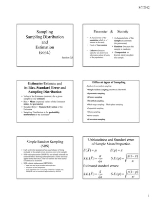
          Sampling                                                                    Parameter &                    Statistic
     Sampling Distribution                                                    • A characteristic of the        • A characteristic of the
                                                                                population which is of           sample (to estimate
              and                                                               interest in the study
                                                                                                                 the parameter)
                                                                              • Fixed or Non-random
         Estimation                                                                                            • Random (because the
                                                                                                                 sample is random)
                                                                              • Unknown (because
            (cont.)                                                             typically you don’t have
                                                                                information about all units
                                                                                                               • Computable or
                                                                                                                 known once you draw
                                                              Session XI        of the population)               the sample


       Estimator/Estimate and                                                       Different types of Sampling
                                                                             Random & nonrandom sampling
   its Bias, Standard Error and                                                Simple random sampling: SRSWR & SRSWOR
       Sampling Distribution                                                   Systematic sampling
• Value of the Estimator (statistic) for a given                               Cluster sampling.
  sample is your estimate
• Bias = Mean (expected value) of the Estimator                                Stratified sampling
  minus the parameter                                                          Multi-stage sampling - Multi-phase sampling
• Standard Error = Standard deviation of the
                                                                               Sequential sampling
  Estimator
• Sampling Distribution is the probability                                     Quota sampling
  distribution of the Estimator                                                Panel samples

                                                                     3         Convenient sampling


                                                                               Unbiasedness and Standard error
      Simple Random Sampling
                                                                                 of Sample Mean/Proportion
               (SRS)
• Each unit in the population has equal chance of being
  included in the sample (even position-wise in the sample)
                                                                           E( X ) = µ                         E ( p) = π
• SRS with replacement (SRSWR): unit already selected are
  returned before drawing subsequent ones. (Same unit may                                   σ                                   π (1 − π )
  appear more than once). Not too realistic but most useful                S .E.( X ) =                       S .E.( p ) =
  for theoretical treatment
                                                                                       n                                             n
• SRS without replacement (SRSWOR):
   – same unit may not be included more than once
   – selections are not independent
                                                                           Estimated standard errors:
   – if the population size is very large compared to sample size,
     SRSWOR can be considered/approximated by SRSWR
                                                                                               S                                 p (1 − p )
                                                                           S .E.( X ) =                       S .E.( p ) =
                                                                                                n                                    n     6


                                                                                                                                                     1
8/7/2012


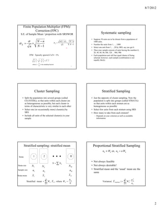
       Finite Population Multiplier (FPM)/
                Correction (FPC)
   S.E. of Sample Mean / proportion with SRSWOR                                                 Systematic sampling
                                                                                     • Suppose 50 units are to be chosen from a population of
           N −nσ                                             π (1 − π )       N −n     1000 units.
  σX =   ×                                            σp =
                                                                 n
                                                                          ×
                                                                              N −1   • Number the units from 1,…, 1000
       n   N −1                                                                      • Select one unit from 1,…,20 by SRS, say you get 6.
                                                                          ?
                                                                                     • Then your sample consists of units having the numbers 6,
                                                                                       26, 46, 66, 86,106, 126….966, 986
                FPM : Typically ignored if n/N < 5%                                  • Each population unit still has equal chance of being
                                                                                       selected; however, each sample (combination is not
                    N −n         n −1                                                  equally likely)
                           = 1−        ≈ 1− f
                    N −1         N −1
                             n
                   where f =   is the sampling fraction
                             N                                                 7


                      Cluster Sampling                                                           Stratified Sampling
     • Split the population into several groups (called                              • Just the opposite of cluster sampling. Now the
       CLUSTERs), so that units within each cluster are                                population is split into groups (called STRATA)
       as heterogeneous as possible, but each cluster in                               so that units within each stratum are as
       terms of characteristic is very similar to each other                           homogeneous as possible
     • Select one (or occasionally more) cluster(s) by                               • Select few units from each stratum using SRS
       SRS                                                                           • How many to take from each stratum?
     • Include all units of the selected cluster(s) in your                             – Depends on your criterion as well as available
       sample                                                                             information


          Stratified sampling: stratified mean                                        Proportional Stratified Sampling
                                                                                                  nh ∝ Wh or, nh = n Wh

 Strata             1                2                                        H

                                                                                     • Not always feasible
                                                    N = ∑ Nh
Strata size        N1              N2                                         NH     • Not always desirable!
Sample size        n1                                                         nH     • Stratified mean and the ‘usual’ mean are the
                                    n2
                                                                                       same
Strata mean        X1               X2                                        XH
                                         H                                                                                   H         2
                                                                              Nh                                                      σh
              Stratified mean = ∑ W h X h , where W h =                                           Variance( X stratified ) = ∑ W h2
                                         h =1                                 N                                              h =1     nh


                                                                                                                                                        2
8/7/2012


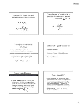
                                                                                               Determination of sample size in
            Best choice of sample size when
                                                                                               stratified sampling with budget
           strata variation is known/estimable
                                                                                                           constraint ∑ c j n j ≤ B

                                       nh ∝ N h σ h
                                                                                                                         N jσ j
                                                       Wh σ h                                                nj ∝
                                nh = n                                                                                        cj
                                                       ∑Wi σ i


                        Examples of Parameters
                                                                                                Criterion for ‘good’ Estimators
                             of interest
µ = average monthly budget on entertainment                                                   • Unbiased Estimator
π=proportion interested in buying the new model of piano

Understand the estimation problem in the context of stratified sampling                       • Minimum Variance Unbiased Estimator
                H                                                 H          H
                                                     Nh
        µ = ∑ Wh µ h , where Wh =                       . So µ = ∑ Wh µ h = ∑ Wh X h
                                                             ˆ        ˆ                       • Consistent Estimator
               h =1                                  N           h =1       h =1


                                 H                            H              H
                         π = ∑ Wh π h . So π = ∑ Wh π h = ∑ Wh ph
                                            ˆ        ˆ
                                h =1                         h =1            h =1


                      Central Limit Theorem
                                                                                                            Notes about CLT
http://www.statisticalengineering.com/central_limit_theorem_(triangle).htm


                                                                                              • The real strength of the CLT lies with the fact that the
                                                                                                approximation is valid for sampling from ANY population.
        If a large number (typically n≥30) of units                                           • For certain populations, the approximation will be good
           are drawn by SRSWR from a population                                                 even for smaller sample sizes. Typically, of course, the
           (with any probability distribution), then the                                        exact sampling distribution of X depends on the
                                                                                                population probability distribution. If the population is
           sampling(probability) distribution of the                                            normal, then X has a normal distribution for any sample
           sample mean can be approximated by a                                                 size n.
                                                                                                                                                     σ2
           normal distribution, i.e. σ 2                                                      • It is easy to see that   E ( X ) = µ and Var ( X ) =
                                                                                                                                                     n
                                             X → N (µ ,                              )          You do not need CLT for that.
                                                                                 n       17                                                            18


                                                                                                                                                                  3
8/7/2012


            Confidence Interval of µ
                                                                                                                     Problem
                             (σ known)
            0.95 = P[−1.96 < Z < 1.96]                                                      Chief of Police Kathy Ackert has recently instituted a crack-
                                   X −µ                                                     -down on drug dealers in her city. Since the crackdown began,
                  = P[−1.96 <                  < 1.96]
                                   σ                                                        750 of the 12,368 drug dealers in the city have been caught.
                                           n
                                                                                            The mean dollar value of drugs found on these 750 dealers is
                              σ                              σ                              $250,000. The standard deviation of the dollar value of drugs
                  = P[−1.96         < X − µ < 1.96               ]
                                n                            n                              for these 750 dealers is $41,000. Construct for Chief Ackert a
                                    σ                            σ                           90 percent confidence interval for the mean dollar value of
                  = P[ X − 1.96            < µ < X + 1.96                ]
                                       n                             n                      drugs possessed by the city’s drug dealers.
  So, 100(1-α)% C.I. for µ is :                                  σ               Standard
                                        X       ± Zα ×                           error
                                                         2           n
                    pt. estimate                                                     19                                                             20
                                                table-value


                           Solution                                                                                  Solution
Want 90% C.I. for µ based on                                                                 Want 90% C.I. for µ based on
           X = 250 K , n = 750 ,                 S = 41 K
                                                                                                  X = 250 K , n = 750, N = 12368, S = 41K
           So the C . I . is
                                                                                                  So the C.I . is
                             41
           250 ± 1 . 645                                                                                        41    12368 − 750
                             750                                                                  250 ± 1.645       ×
                                                                                                                750     12367
 Question: Is it o.k. to replace σ by S?
                                                                                                  = ( 247.62, 252.38)
Answer: yes, when the sample size n is large.(because S is a
consistent estimator of σ.

                                                                                     21                                                             22
  Strictly speaking, we should be using FPM here!


                                                                                                          Correct interpretation of
     Interesting observations about C.I.
                                   P[247.62 < µ < 252.38] = 0.90
                                                                                                             confidence level
   • Interpretation of the confidence
     coefficient/level
       – how should we interpret the probability
         statement? (confidence coefficient)
   • Link between                                                                σ
       – confidence coefficient/level                    L = 2 zα
       – accuracy (length of the C.I.)                                       2       n
       – sample size
                                                                                 σ                                          µ
                                                         H = zα
                                                                         2       n   23                                                             24


                                                                                                                                                                   4
8/7/2012


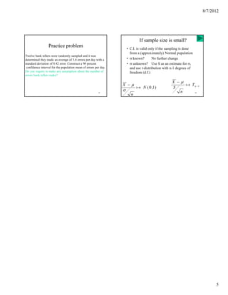
                                                                              If sample size is small?
                  Practice problem                                    • C.I. is valid only if the sampling is done
                                                                        from a (approximately) Normal population
Twelve bank tellers were randomly sampled and it was
determined they made an average of 3.6 errors per day with a          • σ known?        No further change
standard deviation of 0.42 error. Construct a 90 percent              • σ unknown? Use S as an estimate for σ,
 confidence interval for the population mean of errors per day.         and use t-distribution with n-1 degrees of
Do you require to make any assumption about the number of               freedom (d.f.)
errors bank tellers make?

                                                                                                    X −µ
                                                                  X −µ                                   ֏ T n −1
                                                                            ֏ N ( 0 ,1)             S
                                                         25
                                                                  σ                                    n             26
                                                                        n


                                                                                                                                5

More Related Content

Similar to Session 11 12

Introduction to sampling
Introduction to samplingIntroduction to sampling
Introduction to samplingSituo Liu
 
AI 바이오 (2_3일차).pdf
AI 바이오 (2_3일차).pdfAI 바이오 (2_3일차).pdf
AI 바이오 (2_3일차).pdf
H K Yoon
 
Resampling methods
Resampling methodsResampling methods
Resampling methods
Setia Pramana
 
Sampling_-_Basic_Concepts_-_Recap (1).ppt
Sampling_-_Basic_Concepts_-_Recap (1).pptSampling_-_Basic_Concepts_-_Recap (1).ppt
Sampling_-_Basic_Concepts_-_Recap (1).ppt
ronaldrobin1
 
Sampling Techniques.pptx
Sampling Techniques.pptxSampling Techniques.pptx
Sampling Techniques.pptx
Mostaque Ahmed
 
Basic Concepts of Non-Parametric Methods ( Statistics )
Basic Concepts of Non-Parametric Methods ( Statistics )Basic Concepts of Non-Parametric Methods ( Statistics )
Basic Concepts of Non-Parametric Methods ( Statistics )
Hasnat Israq
 
Research Respondents.pptx
Research Respondents.pptxResearch Respondents.pptx
Research Respondents.pptx
Cendz Flores
 
Review of Chapters 1-5.ppt
Review of Chapters 1-5.pptReview of Chapters 1-5.ppt
Review of Chapters 1-5.ppt
NobelFFarrar
 
Sampling Theory Part 1
Sampling Theory Part 1Sampling Theory Part 1
Sampling Theory Part 1
FellowBuddy.com
 
Sampling 20 october 2012
Sampling 20 october 2012Sampling 20 october 2012
Sampling 20 october 2012Nurul Ain
 
Biostatistics basics-biostatistics4734
Biostatistics basics-biostatistics4734Biostatistics basics-biostatistics4734
Biostatistics basics-biostatistics4734AbhishekDas15
 
LR 9 Estimation.pdf
LR 9 Estimation.pdfLR 9 Estimation.pdf
LR 9 Estimation.pdf
giovanniealvarez1
 
Predictive analytics
Predictive analyticsPredictive analytics
Predictive analytics
Dinakar nk
 
Weightage & Complex Sampling
Weightage & Complex Sampling Weightage & Complex Sampling
Weightage & Complex Sampling
Azmi Mohd Tamil
 
Random Artificial Incorporation of Noise in a Learning Classifier System Envi...
Random Artificial Incorporation of Noise in a Learning Classifier System Envi...Random Artificial Incorporation of Noise in a Learning Classifier System Envi...
Random Artificial Incorporation of Noise in a Learning Classifier System Envi...
Daniele Loiacono
 
Chapter_2_Sampling.pptx
Chapter_2_Sampling.pptxChapter_2_Sampling.pptx
Chapter_2_Sampling.pptx
SubodhPaudel6
 
2010 smg training_cardiff_day1_session3_higgins
2010 smg training_cardiff_day1_session3_higgins2010 smg training_cardiff_day1_session3_higgins
2010 smg training_cardiff_day1_session3_higginsrgveroniki
 

Similar to Session 11 12 (20)

Introduction to sampling
Introduction to samplingIntroduction to sampling
Introduction to sampling
 
AI 바이오 (2_3일차).pdf
AI 바이오 (2_3일차).pdfAI 바이오 (2_3일차).pdf
AI 바이오 (2_3일차).pdf
 
Resampling methods
Resampling methodsResampling methods
Resampling methods
 
Sampling_-_Basic_Concepts_-_Recap (1).ppt
Sampling_-_Basic_Concepts_-_Recap (1).pptSampling_-_Basic_Concepts_-_Recap (1).ppt
Sampling_-_Basic_Concepts_-_Recap (1).ppt
 
Sampling Techniques.pptx
Sampling Techniques.pptxSampling Techniques.pptx
Sampling Techniques.pptx
 
Basic Concepts of Non-Parametric Methods ( Statistics )
Basic Concepts of Non-Parametric Methods ( Statistics )Basic Concepts of Non-Parametric Methods ( Statistics )
Basic Concepts of Non-Parametric Methods ( Statistics )
 
Research Respondents.pptx
Research Respondents.pptxResearch Respondents.pptx
Research Respondents.pptx
 
Sampling....
Sampling....Sampling....
Sampling....
 
Review of Chapters 1-5.ppt
Review of Chapters 1-5.pptReview of Chapters 1-5.ppt
Review of Chapters 1-5.ppt
 
Sampling Theory Part 1
Sampling Theory Part 1Sampling Theory Part 1
Sampling Theory Part 1
 
Sampling 20 october 2012
Sampling 20 october 2012Sampling 20 october 2012
Sampling 20 october 2012
 
Biostatistics basics-biostatistics4734
Biostatistics basics-biostatistics4734Biostatistics basics-biostatistics4734
Biostatistics basics-biostatistics4734
 
LR 9 Estimation.pdf
LR 9 Estimation.pdfLR 9 Estimation.pdf
LR 9 Estimation.pdf
 
Lecture 5.0 vegetation_sampling
Lecture 5.0 vegetation_samplingLecture 5.0 vegetation_sampling
Lecture 5.0 vegetation_sampling
 
Predictive analytics
Predictive analyticsPredictive analytics
Predictive analytics
 
Weightage & Complex Sampling
Weightage & Complex Sampling Weightage & Complex Sampling
Weightage & Complex Sampling
 
Sampling Design
Sampling DesignSampling Design
Sampling Design
 
Random Artificial Incorporation of Noise in a Learning Classifier System Envi...
Random Artificial Incorporation of Noise in a Learning Classifier System Envi...Random Artificial Incorporation of Noise in a Learning Classifier System Envi...
Random Artificial Incorporation of Noise in a Learning Classifier System Envi...
 
Chapter_2_Sampling.pptx
Chapter_2_Sampling.pptxChapter_2_Sampling.pptx
Chapter_2_Sampling.pptx
 
2010 smg training_cardiff_day1_session3_higgins
2010 smg training_cardiff_day1_session3_higgins2010 smg training_cardiff_day1_session3_higgins
2010 smg training_cardiff_day1_session3_higgins
 

More from vivek_shaw

Lecture 11 market structure- perfect competition
Lecture 11  market structure- perfect competitionLecture 11  market structure- perfect competition
Lecture 11 market structure- perfect competitionvivek_shaw
 
Lecture 9 costs
Lecture 9  costsLecture 9  costs
Lecture 9 costsvivek_shaw
 
Lecture 8 production, optimal inputs
Lecture 8  production, optimal inputsLecture 8  production, optimal inputs
Lecture 8 production, optimal inputsvivek_shaw
 
Lecture 8 production, optimal inputs (1)
Lecture 8  production, optimal inputs (1)Lecture 8  production, optimal inputs (1)
Lecture 8 production, optimal inputs (1)vivek_shaw
 
Lecture 3 dds sand elasticity
Lecture 3  dds sand elasticityLecture 3  dds sand elasticity
Lecture 3 dds sand elasticityvivek_shaw
 
Consumertheory1
Consumertheory1Consumertheory1
Consumertheory1vivek_shaw
 
Consumer theory 2
Consumer theory 2Consumer theory 2
Consumer theory 2vivek_shaw
 
Class2 market, demand and supply
Class2  market, demand and supplyClass2  market, demand and supply
Class2 market, demand and supplyvivek_shaw
 
Policy implications
Policy implicationsPolicy implications
Policy implicationsvivek_shaw
 
Man org session 3-org and technology_5th july 2012
Man org session 3-org and technology_5th july 2012Man org session 3-org and technology_5th july 2012
Man org session 3-org and technology_5th july 2012vivek_shaw
 
Man org session 14_org decision making_16th august 2012
Man org session 14_org decision making_16th august 2012Man org session 14_org decision making_16th august 2012
Man org session 14_org decision making_16th august 2012vivek_shaw
 
Man org session 12_org learning_3rd august 2012
Man org session 12_org learning_3rd august 2012Man org session 12_org learning_3rd august 2012
Man org session 12_org learning_3rd august 2012vivek_shaw
 
Man org session 11 interorganizational relationships_2nd august 2012
Man org session 11 interorganizational relationships_2nd august 2012Man org session 11 interorganizational relationships_2nd august 2012
Man org session 11 interorganizational relationships_2nd august 2012vivek_shaw
 
Man org session 10_org control_27th july 2012
Man org session 10_org control_27th july 2012Man org session 10_org control_27th july 2012
Man org session 10_org control_27th july 2012vivek_shaw
 

More from vivek_shaw (20)

Lecture 11 market structure- perfect competition
Lecture 11  market structure- perfect competitionLecture 11  market structure- perfect competition
Lecture 11 market structure- perfect competition
 
Lecture 9 costs
Lecture 9  costsLecture 9  costs
Lecture 9 costs
 
Lecture 8 production, optimal inputs
Lecture 8  production, optimal inputsLecture 8  production, optimal inputs
Lecture 8 production, optimal inputs
 
Lecture 8 production, optimal inputs (1)
Lecture 8  production, optimal inputs (1)Lecture 8  production, optimal inputs (1)
Lecture 8 production, optimal inputs (1)
 
Lecture 3 dds sand elasticity
Lecture 3  dds sand elasticityLecture 3  dds sand elasticity
Lecture 3 dds sand elasticity
 
Game theory 3
Game theory 3Game theory 3
Game theory 3
 
Game theory 1
Game theory 1Game theory 1
Game theory 1
 
Game theory 2
Game theory 2Game theory 2
Game theory 2
 
Ford motors
Ford motorsFord motors
Ford motors
 
Consumertheory1
Consumertheory1Consumertheory1
Consumertheory1
 
Consumer theory 2
Consumer theory 2Consumer theory 2
Consumer theory 2
 
Class2 market, demand and supply
Class2  market, demand and supplyClass2  market, demand and supply
Class2 market, demand and supply
 
Auctions 1
Auctions 1Auctions 1
Auctions 1
 
Costs2
Costs2Costs2
Costs2
 
Policy implications
Policy implicationsPolicy implications
Policy implications
 
Man org session 3-org and technology_5th july 2012
Man org session 3-org and technology_5th july 2012Man org session 3-org and technology_5th july 2012
Man org session 3-org and technology_5th july 2012
 
Man org session 14_org decision making_16th august 2012
Man org session 14_org decision making_16th august 2012Man org session 14_org decision making_16th august 2012
Man org session 14_org decision making_16th august 2012
 
Man org session 12_org learning_3rd august 2012
Man org session 12_org learning_3rd august 2012Man org session 12_org learning_3rd august 2012
Man org session 12_org learning_3rd august 2012
 
Man org session 11 interorganizational relationships_2nd august 2012
Man org session 11 interorganizational relationships_2nd august 2012Man org session 11 interorganizational relationships_2nd august 2012
Man org session 11 interorganizational relationships_2nd august 2012
 
Man org session 10_org control_27th july 2012
Man org session 10_org control_27th july 2012Man org session 10_org control_27th july 2012
Man org session 10_org control_27th july 2012
 

Session 11 12

  • 1. 8/7/2012 Sampling Parameter & Statistic Sampling Distribution • A characteristic of the • A characteristic of the population which is of sample (to estimate and interest in the study the parameter) • Fixed or Non-random Estimation • Random (because the sample is random) • Unknown (because (cont.) typically you don’t have information about all units • Computable or known once you draw Session XI of the population) the sample Estimator/Estimate and Different types of Sampling Random & nonrandom sampling its Bias, Standard Error and Simple random sampling: SRSWR & SRSWOR Sampling Distribution Systematic sampling • Value of the Estimator (statistic) for a given Cluster sampling. sample is your estimate • Bias = Mean (expected value) of the Estimator Stratified sampling minus the parameter Multi-stage sampling - Multi-phase sampling • Standard Error = Standard deviation of the Sequential sampling Estimator • Sampling Distribution is the probability Quota sampling distribution of the Estimator Panel samples 3 Convenient sampling Unbiasedness and Standard error Simple Random Sampling of Sample Mean/Proportion (SRS) • Each unit in the population has equal chance of being included in the sample (even position-wise in the sample) E( X ) = µ E ( p) = π • SRS with replacement (SRSWR): unit already selected are returned before drawing subsequent ones. (Same unit may σ π (1 − π ) appear more than once). Not too realistic but most useful S .E.( X ) = S .E.( p ) = for theoretical treatment n n • SRS without replacement (SRSWOR): – same unit may not be included more than once – selections are not independent Estimated standard errors: – if the population size is very large compared to sample size, SRSWOR can be considered/approximated by SRSWR S p (1 − p ) S .E.( X ) = S .E.( p ) = n n 6 1
  • 2. 8/7/2012 Finite Population Multiplier (FPM)/ Correction (FPC) S.E. of Sample Mean / proportion with SRSWOR Systematic sampling • Suppose 50 units are to be chosen from a population of N −nσ π (1 − π ) N −n 1000 units. σX = × σp = n × N −1 • Number the units from 1,…, 1000 n N −1 • Select one unit from 1,…,20 by SRS, say you get 6. ? • Then your sample consists of units having the numbers 6, 26, 46, 66, 86,106, 126….966, 986 FPM : Typically ignored if n/N < 5% • Each population unit still has equal chance of being selected; however, each sample (combination is not N −n n −1 equally likely) = 1− ≈ 1− f N −1 N −1 n where f = is the sampling fraction N 7 Cluster Sampling Stratified Sampling • Split the population into several groups (called • Just the opposite of cluster sampling. Now the CLUSTERs), so that units within each cluster are population is split into groups (called STRATA) as heterogeneous as possible, but each cluster in so that units within each stratum are as terms of characteristic is very similar to each other homogeneous as possible • Select one (or occasionally more) cluster(s) by • Select few units from each stratum using SRS SRS • How many to take from each stratum? • Include all units of the selected cluster(s) in your – Depends on your criterion as well as available sample information Stratified sampling: stratified mean Proportional Stratified Sampling nh ∝ Wh or, nh = n Wh Strata 1 2 H • Not always feasible N = ∑ Nh Strata size N1 N2 NH • Not always desirable! Sample size n1 nH • Stratified mean and the ‘usual’ mean are the n2 same Strata mean X1 X2 XH H H 2 Nh σh Stratified mean = ∑ W h X h , where W h = Variance( X stratified ) = ∑ W h2 h =1 N h =1 nh 2
  • 3. 8/7/2012 Determination of sample size in Best choice of sample size when stratified sampling with budget strata variation is known/estimable constraint ∑ c j n j ≤ B nh ∝ N h σ h N jσ j Wh σ h nj ∝ nh = n cj ∑Wi σ i Examples of Parameters Criterion for ‘good’ Estimators of interest µ = average monthly budget on entertainment • Unbiased Estimator π=proportion interested in buying the new model of piano Understand the estimation problem in the context of stratified sampling • Minimum Variance Unbiased Estimator H H H Nh µ = ∑ Wh µ h , where Wh = . So µ = ∑ Wh µ h = ∑ Wh X h ˆ ˆ • Consistent Estimator h =1 N h =1 h =1 H H H π = ∑ Wh π h . So π = ∑ Wh π h = ∑ Wh ph ˆ ˆ h =1 h =1 h =1 Central Limit Theorem Notes about CLT http://www.statisticalengineering.com/central_limit_theorem_(triangle).htm http://www.statisticalengineering.com/central_limit_theorem_(triangle).htm • The real strength of the CLT lies with the fact that the approximation is valid for sampling from ANY population. If a large number (typically n≥30) of units • For certain populations, the approximation will be good are drawn by SRSWR from a population even for smaller sample sizes. Typically, of course, the (with any probability distribution), then the exact sampling distribution of X depends on the population probability distribution. If the population is sampling(probability) distribution of the normal, then X has a normal distribution for any sample sample mean can be approximated by a size n. σ2 normal distribution, i.e. σ 2 • It is easy to see that E ( X ) = µ and Var ( X ) = n X → N (µ , ) You do not need CLT for that. n 17 18 3
  • 4. 8/7/2012 Confidence Interval of µ Problem (σ known) 0.95 = P[−1.96 < Z < 1.96] Chief of Police Kathy Ackert has recently instituted a crack- X −µ -down on drug dealers in her city. Since the crackdown began, = P[−1.96 < < 1.96] σ 750 of the 12,368 drug dealers in the city have been caught. n The mean dollar value of drugs found on these 750 dealers is σ σ $250,000. The standard deviation of the dollar value of drugs = P[−1.96 < X − µ < 1.96 ] n n for these 750 dealers is $41,000. Construct for Chief Ackert a σ σ 90 percent confidence interval for the mean dollar value of = P[ X − 1.96 < µ < X + 1.96 ] n n drugs possessed by the city’s drug dealers. So, 100(1-α)% C.I. for µ is : σ Standard X ± Zα × error 2 n pt. estimate 19 20 table-value Solution Solution Want 90% C.I. for µ based on Want 90% C.I. for µ based on X = 250 K , n = 750 , S = 41 K X = 250 K , n = 750, N = 12368, S = 41K So the C . I . is So the C.I . is 41 250 ± 1 . 645 41 12368 − 750 750 250 ± 1.645 × 750 12367 Question: Is it o.k. to replace σ by S? = ( 247.62, 252.38) Answer: yes, when the sample size n is large.(because S is a consistent estimator of σ. 21 22 Strictly speaking, we should be using FPM here! Correct interpretation of Interesting observations about C.I. P[247.62 < µ < 252.38] = 0.90 confidence level • Interpretation of the confidence coefficient/level – how should we interpret the probability statement? (confidence coefficient) • Link between σ – confidence coefficient/level L = 2 zα – accuracy (length of the C.I.) 2 n – sample size σ µ H = zα 2 n 23 24 4
  • 5. 8/7/2012 If sample size is small? Practice problem • C.I. is valid only if the sampling is done from a (approximately) Normal population Twelve bank tellers were randomly sampled and it was determined they made an average of 3.6 errors per day with a • σ known? No further change standard deviation of 0.42 error. Construct a 90 percent • σ unknown? Use S as an estimate for σ, confidence interval for the population mean of errors per day. and use t-distribution with n-1 degrees of Do you require to make any assumption about the number of freedom (d.f.) errors bank tellers make? X −µ X −µ ֏ T n −1 ֏ N ( 0 ,1) S 25 σ n 26 n 5