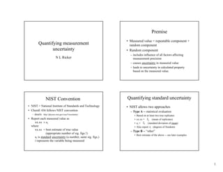
1. Premise
• Measured value = repeatable component +
Quantifying measurement random component
uncertainty • Random component
– includes influence of all factors affecting
N L Ricker measurement precision
– causes uncertainty in measured value
– leads to uncertainty in calculated property
based on the measured value.
NIST Convention Quantifying standard uncertainty
• NIST = National Institute of Standards and Technology • NIST allows two approaches
• ChemE 436 follows NIST convention – Type A -- statistical evaluation
– details: http://physics.nist.gov/cuu/Uncertainty/ • Based on at least two true replicates
• Report each measured value as • xx.xx = xi (mean of replicates)
xx.xx ± ui • ui = si (standard deviation of mean)
where • Also report νi (degrees of freedom)
xx.xx = best estimate of true value – Type B -- “other”
(appropriate number of sig. figs.!)
• Best estimate of the above -- see later examples
ui is standard uncertainty (a number, same sig. figs.)
i represents the variable being measured
1

2. Equations for Type A evaluation Example
ni
Excel function:
Sample 1
Mean
xi = ∑ xi, k Your evaluation of the activated carbon
n i k =1 =AVERAGE( )
adsorption system consists of 4 replicates:
Sample ni
1
Standard
Deviation
si =
n − 1 k =1
( )
∑ xi, k − x i 2 =STDEV( ) k Pin Pout
Mean 1 1030 211
si
Standard si = 2 1220 252
Deviation ni
3 985 197
Degrees of ν i = ni − 1
Freedom 4 1120 237
ni = number of replicates for variable i NOTE: each measured value has 3 significant figures
xi,k = value of kth replicate
Example -- sample standard deviation
Example -- mean value
ni
1
1 ni si = (
∑ xi, k − xi 2) (Excel: STDEV)
xi = ∑ xi, k (Excel’s AVERAGE function) n − 1 k =1
n i k =1
1
1 s Pin = [ (1030 − 1090 ) 2 + (1220 - 1090 )2
x Pin = [1030 + 1220 + 985 + 1120 ] 4 −1
4
+ (985 - 1090 )2 + (1120 - 1090 )2 ]
= 1088.75
= 103.9531
= 1090 (rounded to 3 significant figures
= ROUND(1088.75, -1) ) = 100 (rounded -- one’s digit is not significant)
Similarly
Similarly
x Pout = 224 s Pout = 25 (rounded -- one’s digit is significant)
2

3. Example -- mean standard deviation
si
Example -- reporting results
si =
ni
103 . 9531 Pin Pout
s Pin =
4
= 51.97656 Result 1090 ± 50 224 ± 12
= 50 (rounded -- one’s digit is not significant) D.O.F. 3 3
Similarly
s Pout = 12 (rounded -- one’s digit is significant)
Example Type B evaluation
Type B evaluation
• You are using a thermometer
• Judgment based on: • The manufacturer claims accuracy = ±1 oC.
– data obtained in a similar experiment – Assume: as measured accuracy rating, not a
– known “typical” instrument performance standard uncertainty.
– manufacturer's specifications – Assume the manufacturer has been
– calibration report conservative, so larger errors are very unlikely.
– uncertainties assigned to reference data – Lacking other information, assume all errors in
taken from handbooks this range are equally probable.
– etc.
3

4. Uniform (rectangular) probability Moments of a probability
Probability 1
Example
with
distribution
function
x1 = 1
f(x)
0.5
x2 = 3 • Zeroth moment -- area under f(x):
0 ∞
µ 0 = ∫ f ( x )dx
0 1 2 3 4 −∞
x
Random variable
Formal definition: (measurement) For a rectangular probability distribution:
f (x) = 0 − ∞ < x ≤ x1
1 x1 and x2 represent limits of 1
f (x) = ∞
x 2 − x1
x1 ≤ x ≤ x 2 measurement uncertainty (on both µ 0 = ∫− ∞ f ( x )dx = (x 2 − x1 ) = 1
sides of the measured value) x 2 − x1
f (x) = 0 x2 ≤ x < ∞
First moment (“mean”) Second moment (“variance”)
∞
∫ (x − µ ) f (x )dx
2
∞
∫ xf ( x )dx σ 2
= −∞
µ= −∞ µ0
µ0
For a rectangular distribution:
For a rectangular distribution:
σ2 =
(x2 − x1 )2 (variance)
x +x 12
µ= 1 2 x 2 − x1
2 σ = (standard deviation)
2 3
4

5. Using assumed rectangular Assuming a triangular probability
distribution in Type B evaluation distribution
x 2, i − x1, i f(x)
ui ≈ σ i = Concept: smaller errors more probable
2 3
2
Example: accuracy = ±1 oC implies x 2 − x1
x 2 − x1
σ =
2 6
x 2, i − x1, i 2
ui ≈ σ i = = = 0.58 oC
2 3 2 3 0
x
x1 x x2
Assuming a Normal distribution Comparison
1  1  x − µ 2 
N (µ , σ ) ⇔ f ( x ) = exp −   
σ 2π   x 2, i − x1, i
 2 σ   Rectangular ui ≈ σ i = =
2
= 0.6 (rounded)
1 2 3 2 3
Example: N(µ =1.5, σ = 0.5)
0.8 Note:
xi ,2 − xi,1 2
0.6 Triangular ui ≈ σ i = = = 0.4 (rounded)
x>µ+3σ 2 6 2 6
f(x)
0.4 x<µ−3σ
µ
0.2 µ−σ xi, 2 − xi,1 2
µ+σ
very unlikely! Normal ui ≈ σ i = = = 0.3 (rounded)
0 6 6
0 1 2 3
x Result depends on assumptions. (No “right” answer.)
State and justify your assumptions.
Thus, assume x2 − x1 = 6 σ Rectangular is the most conservative (largest uncertainty).
5