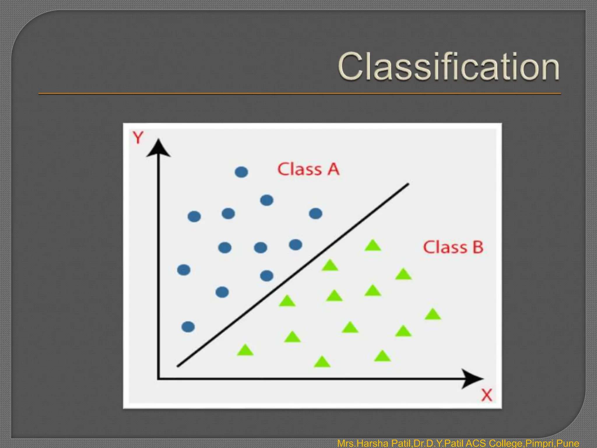
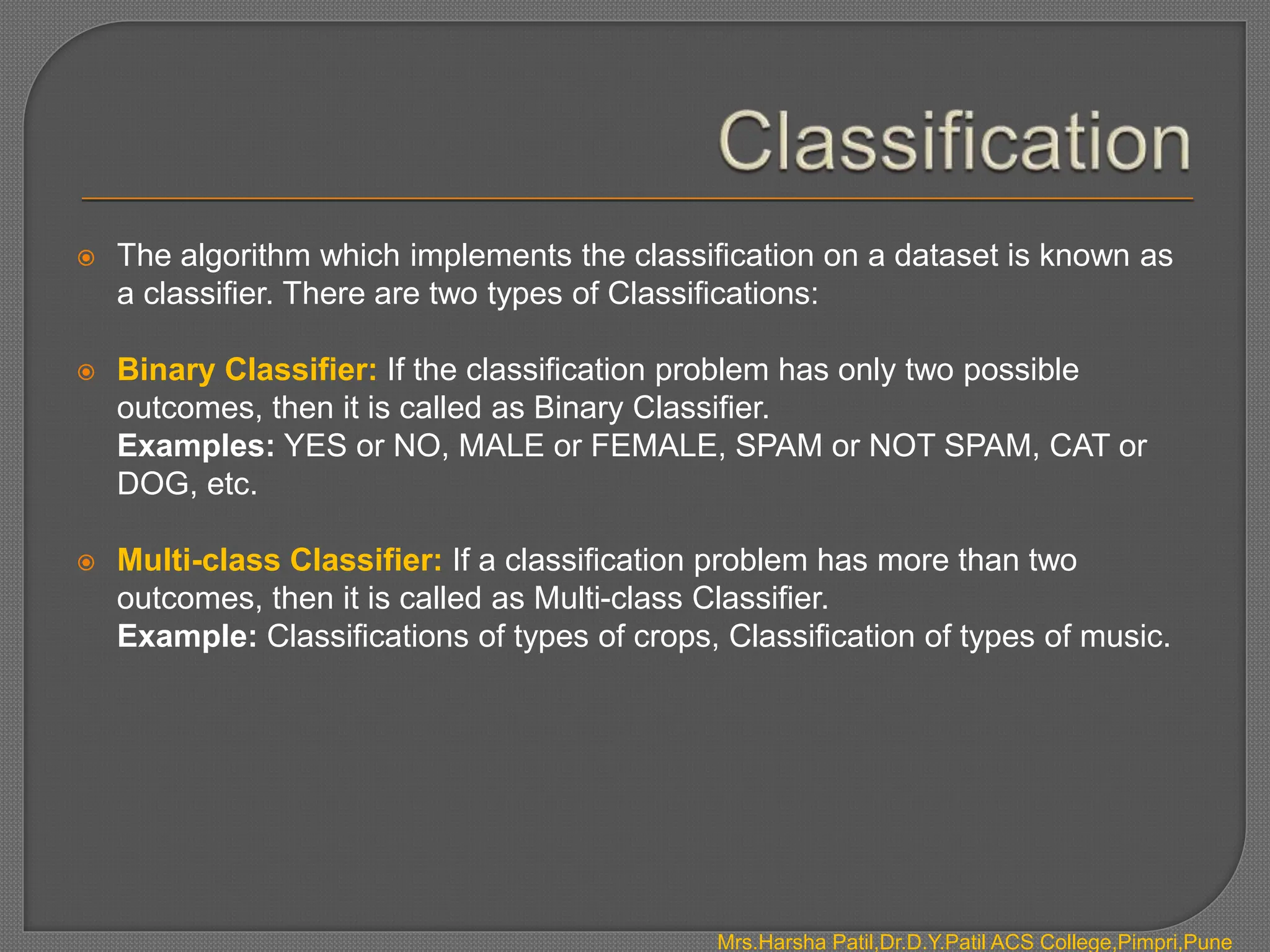
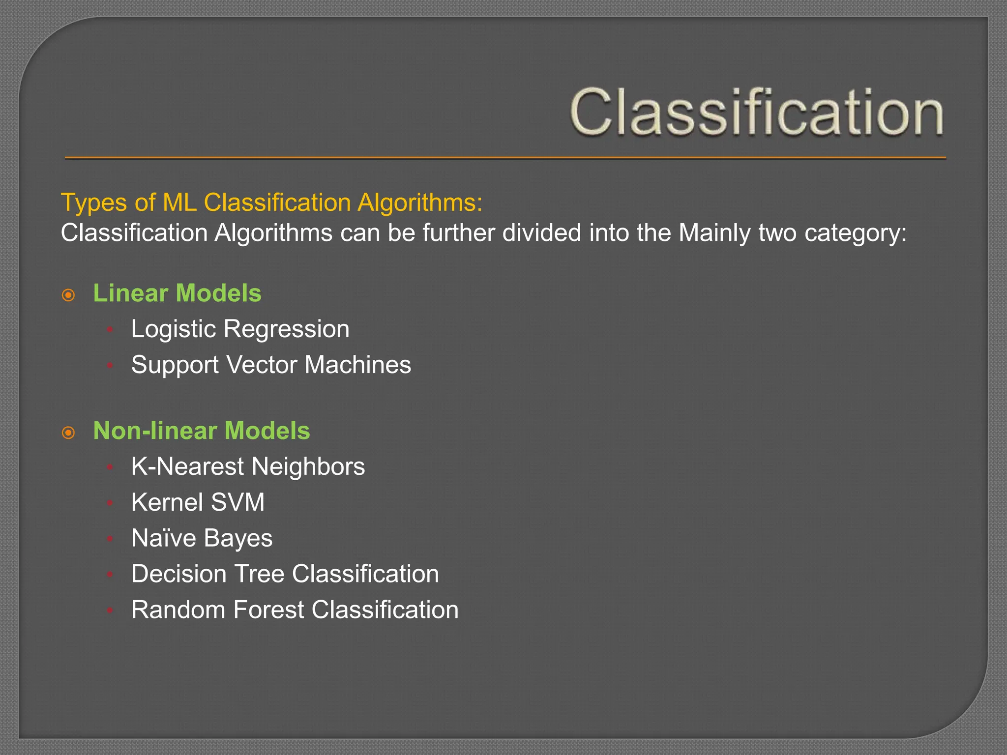
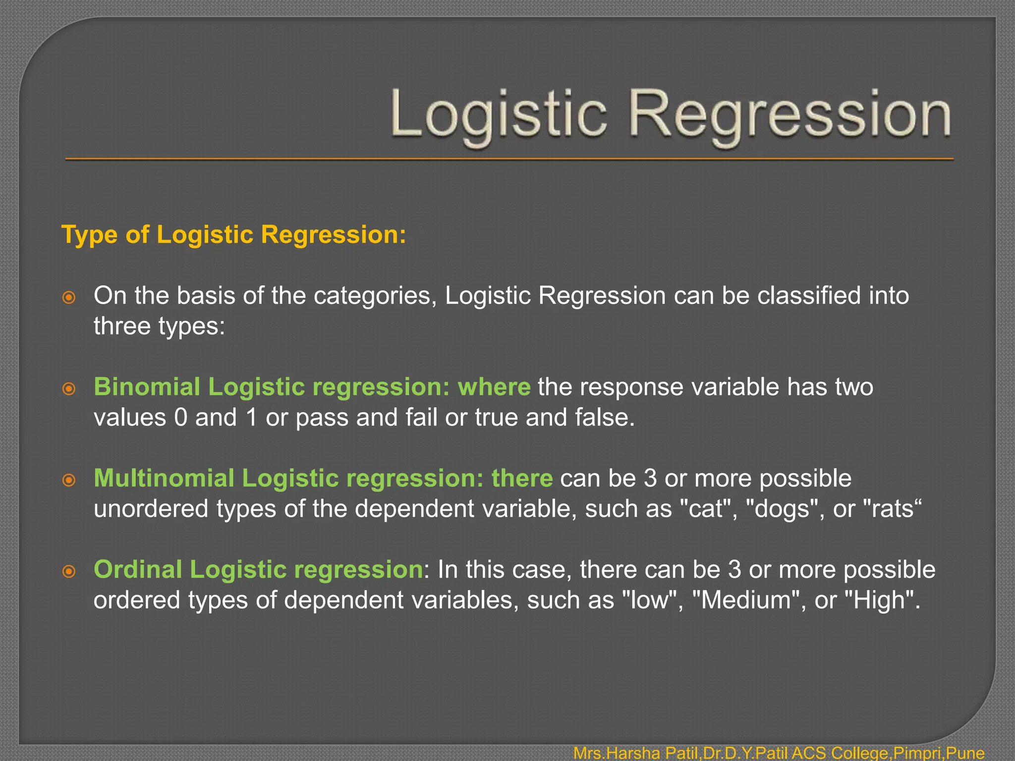
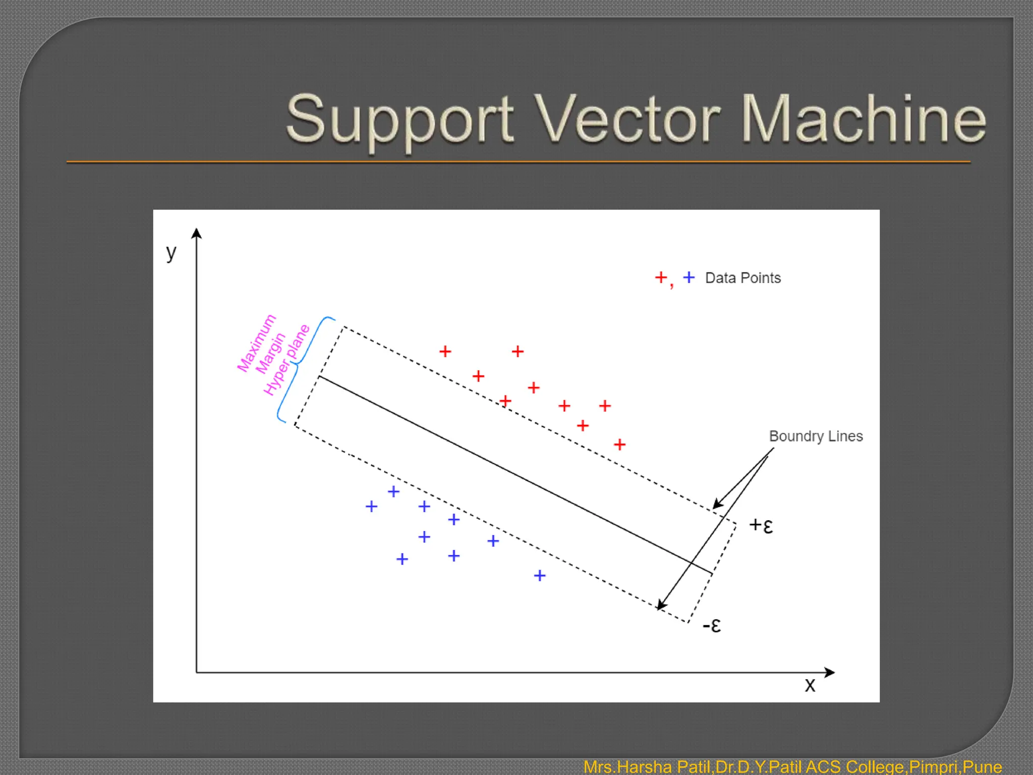
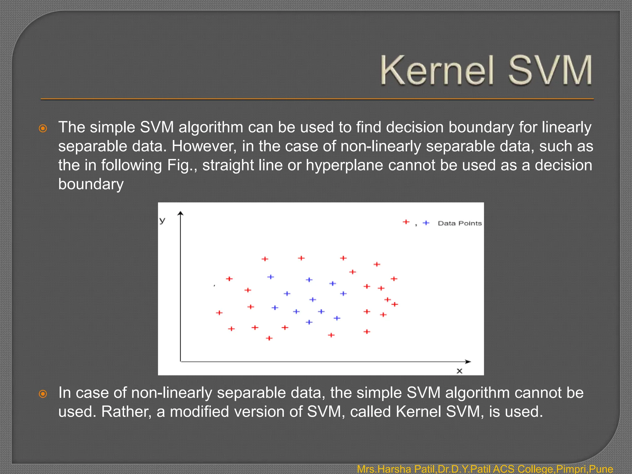
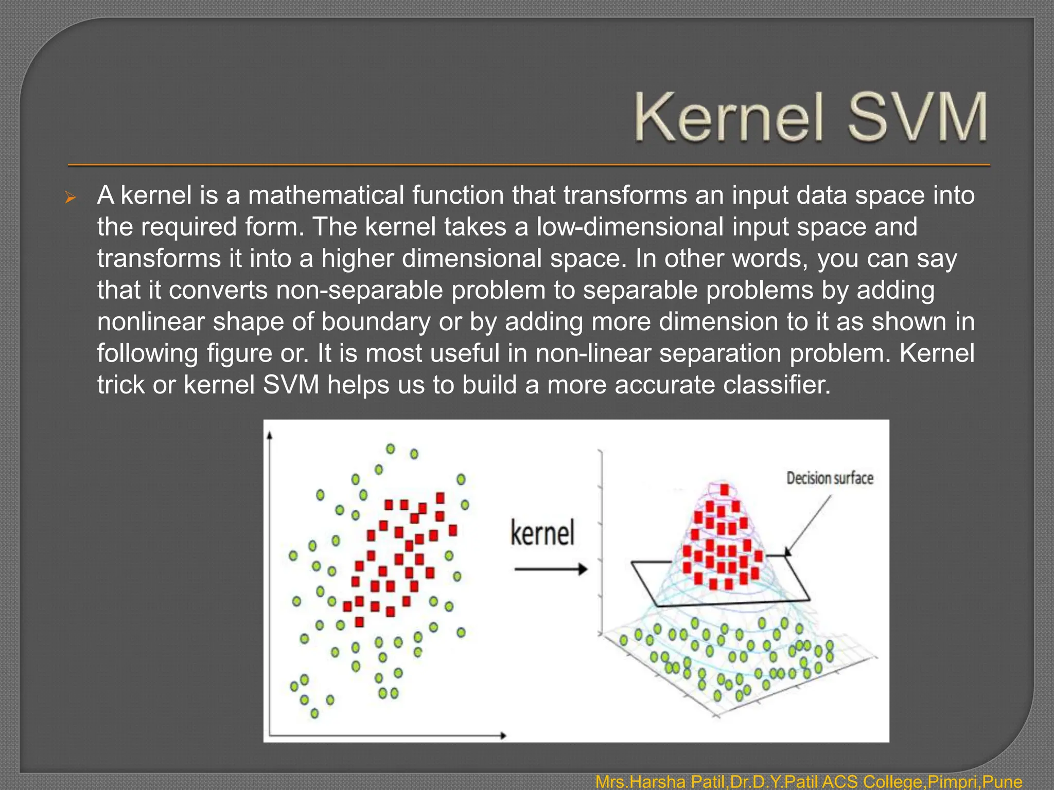
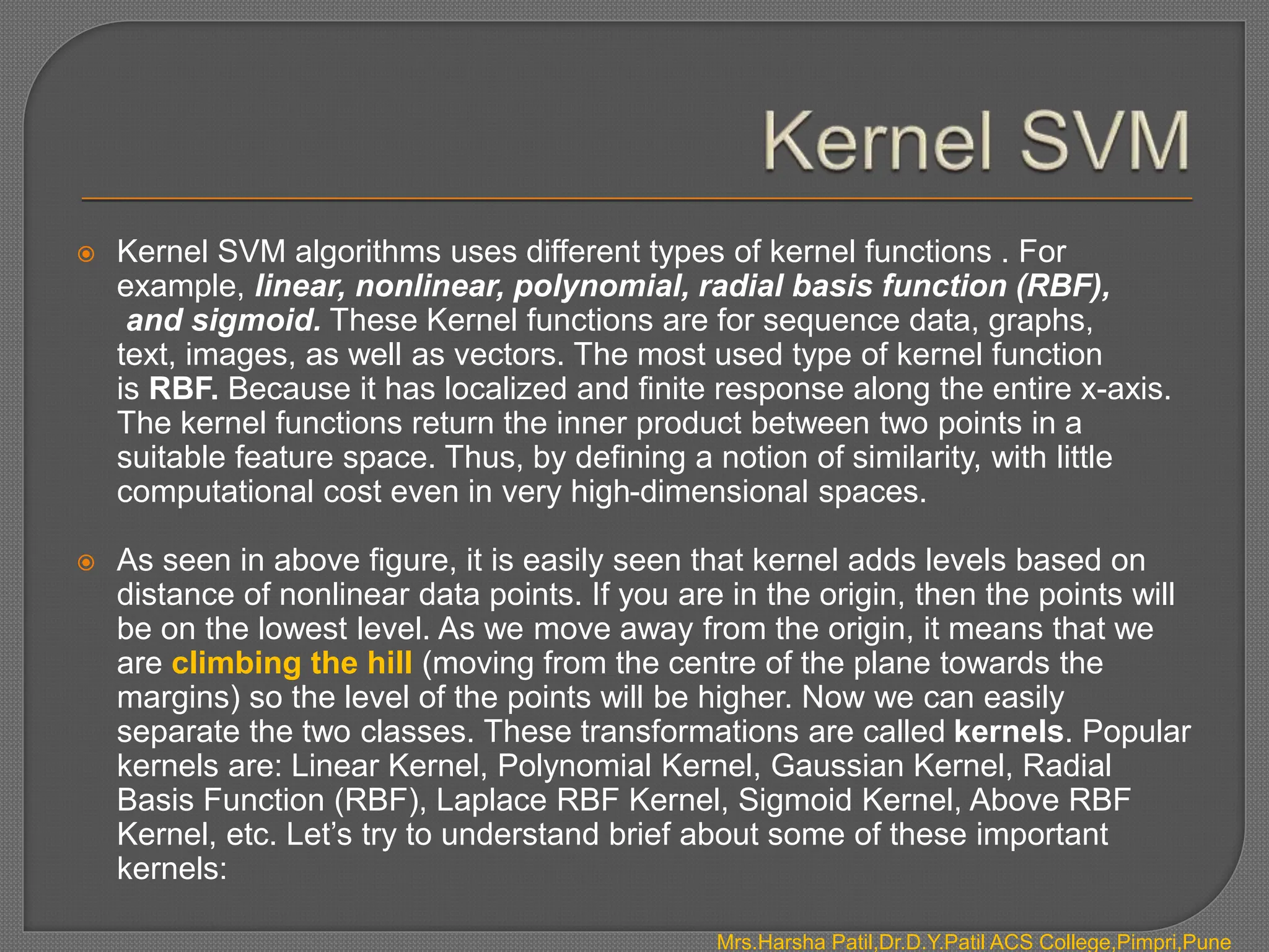
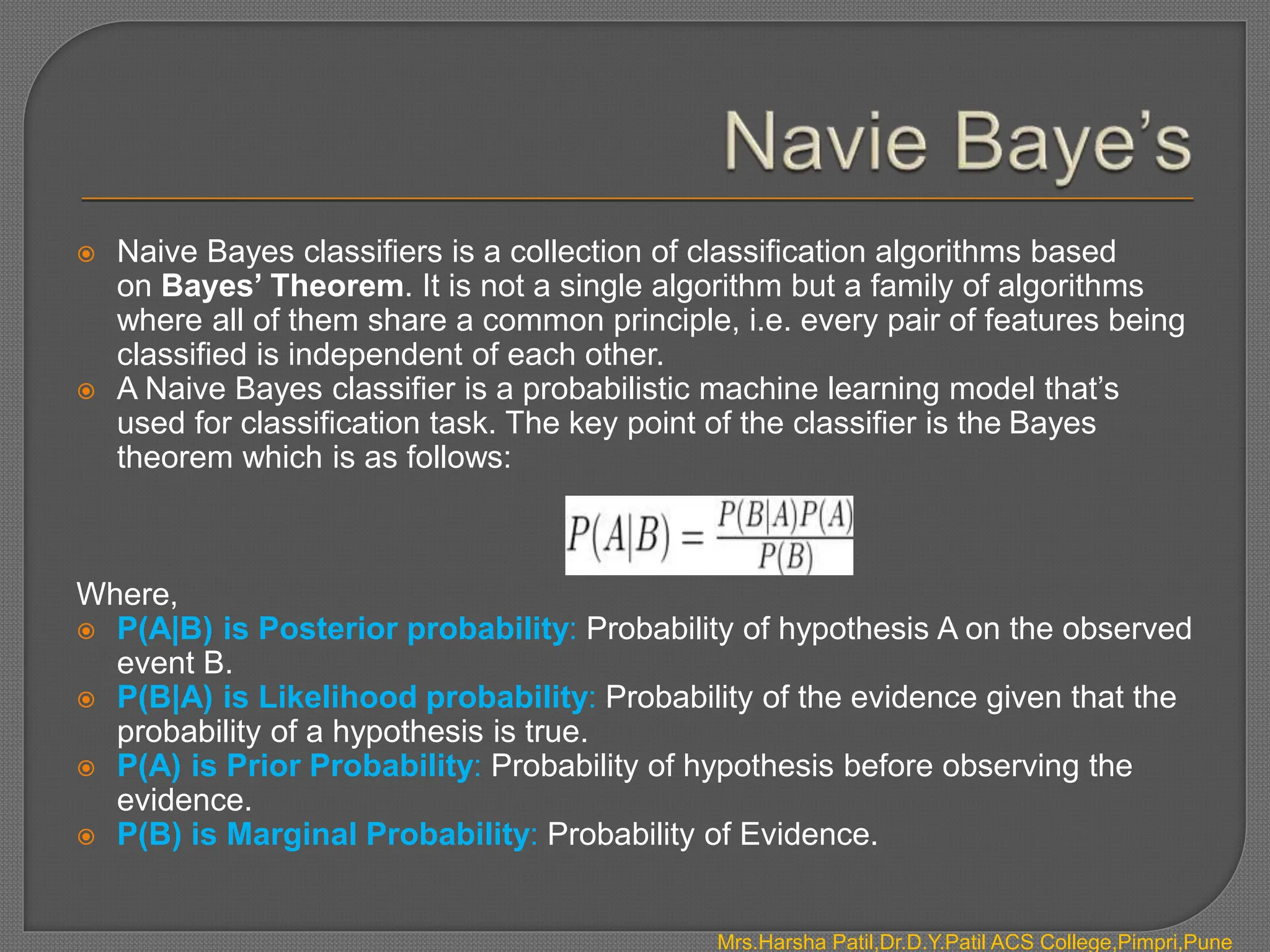
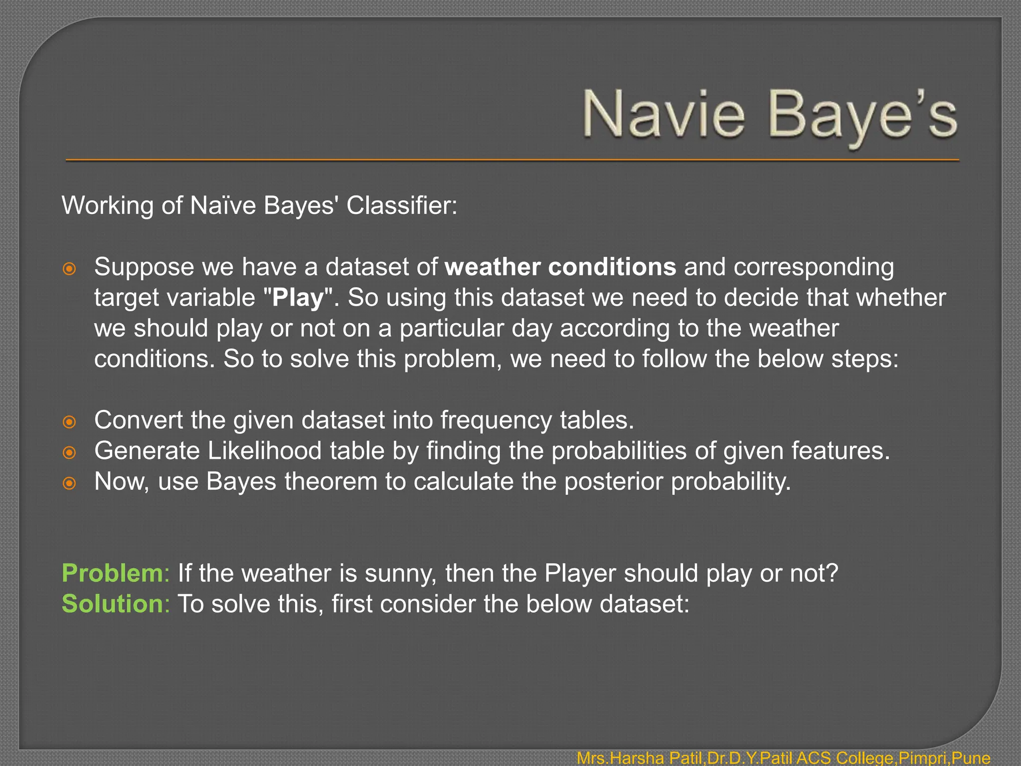
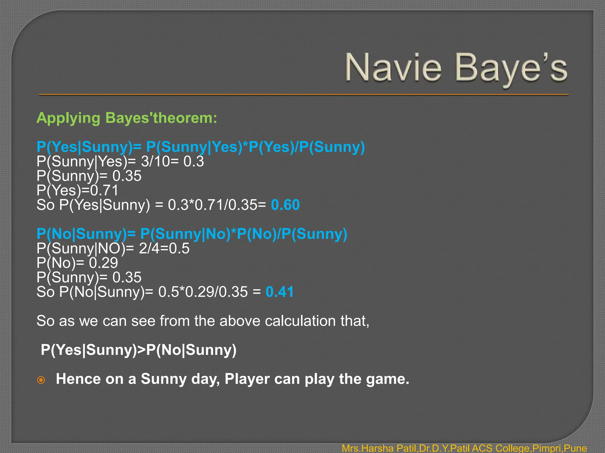
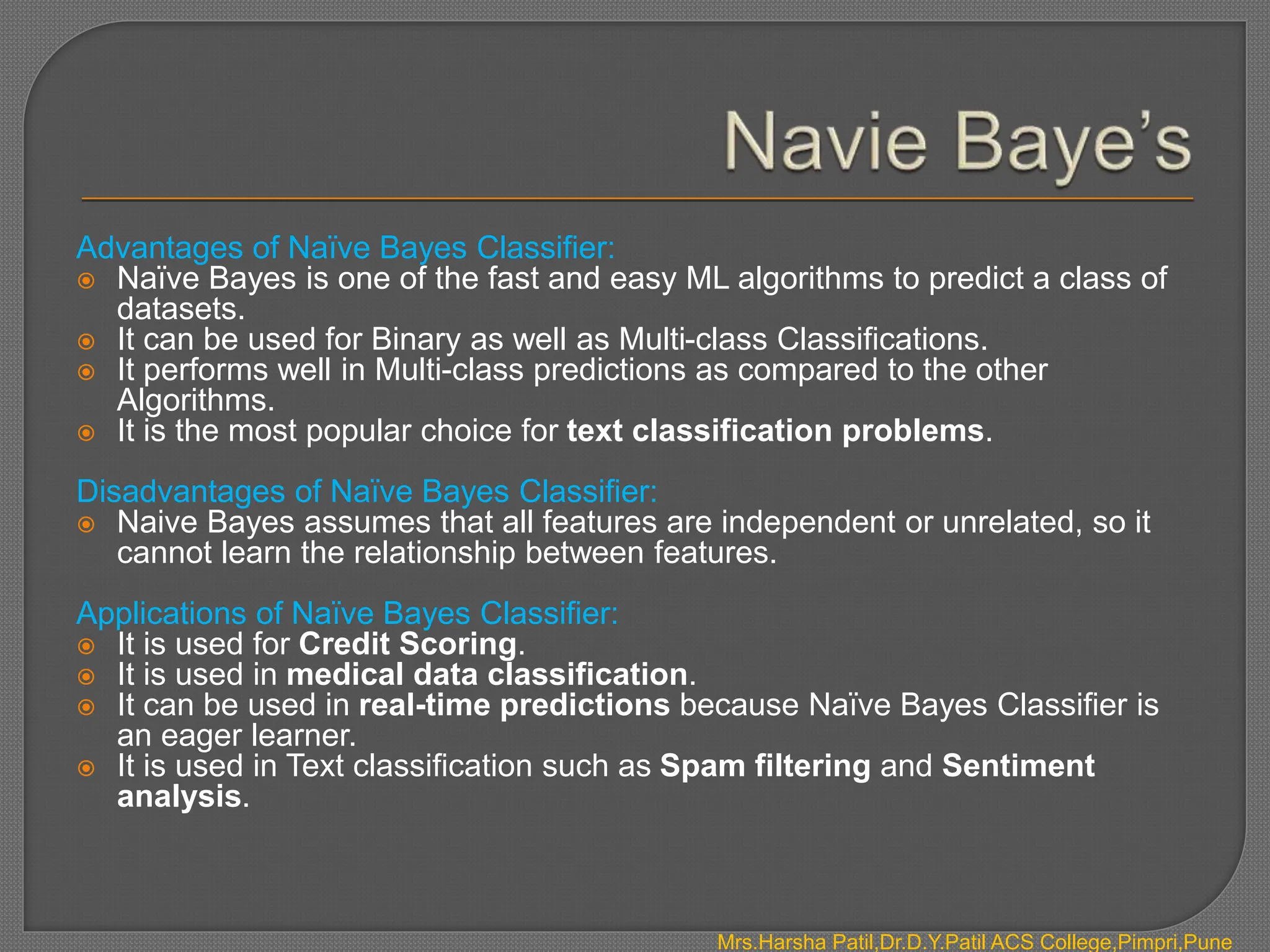
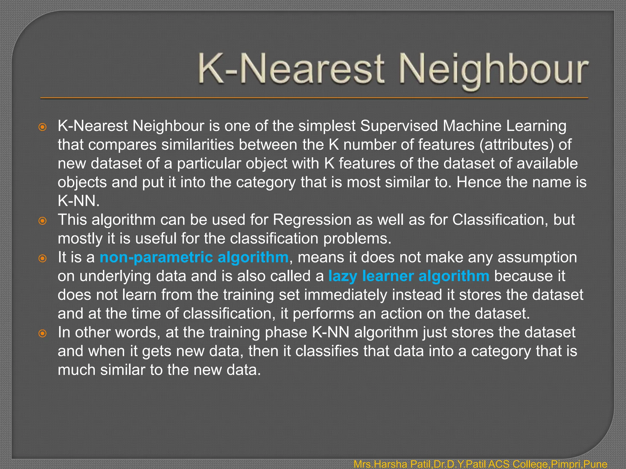
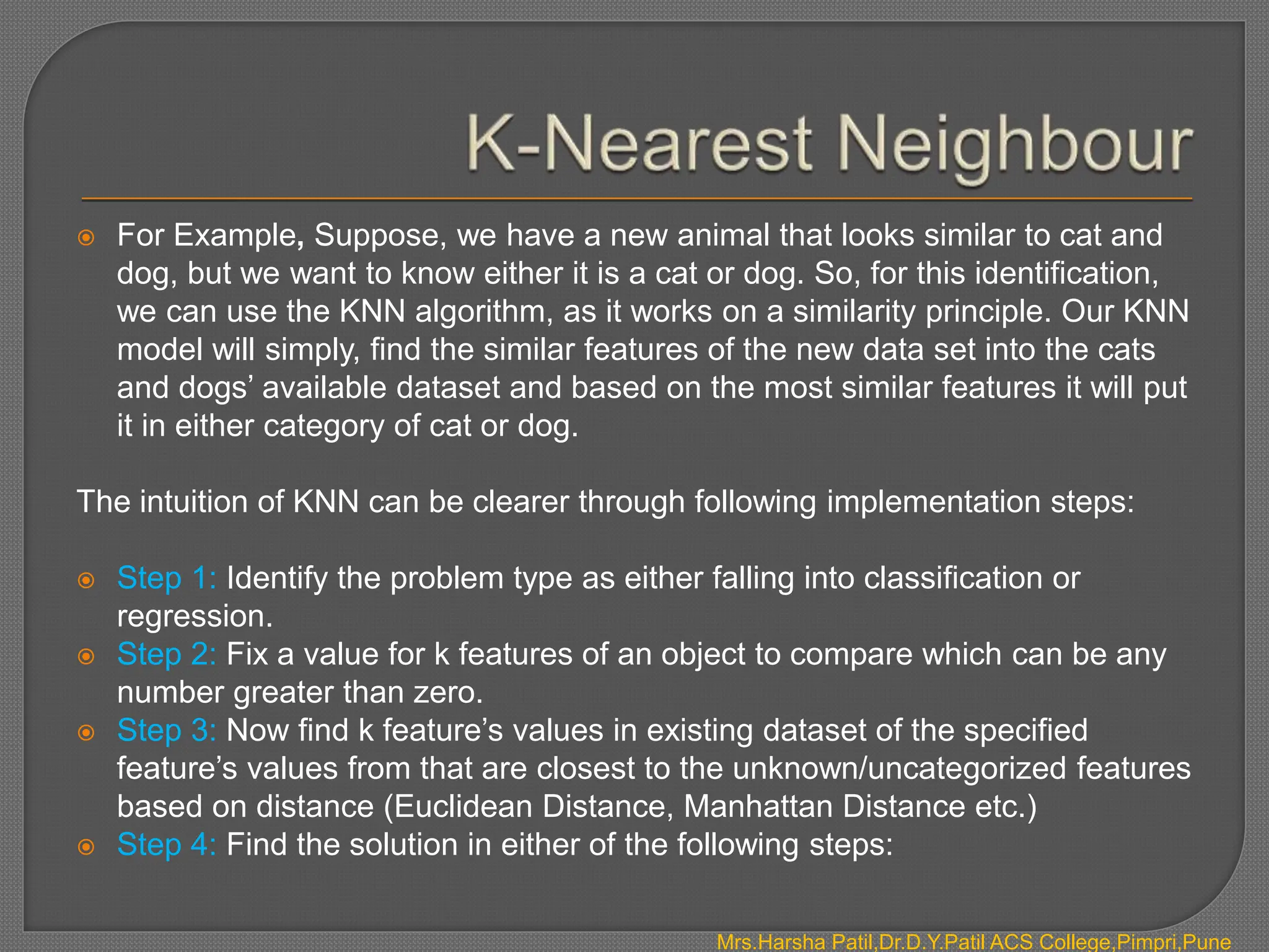
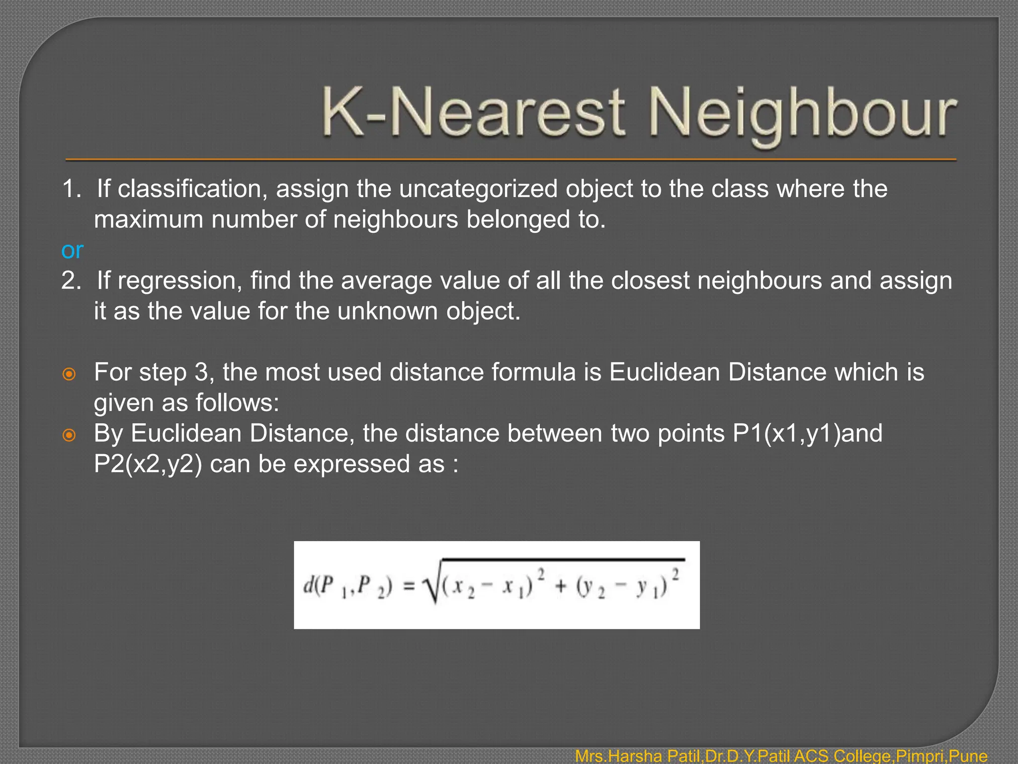
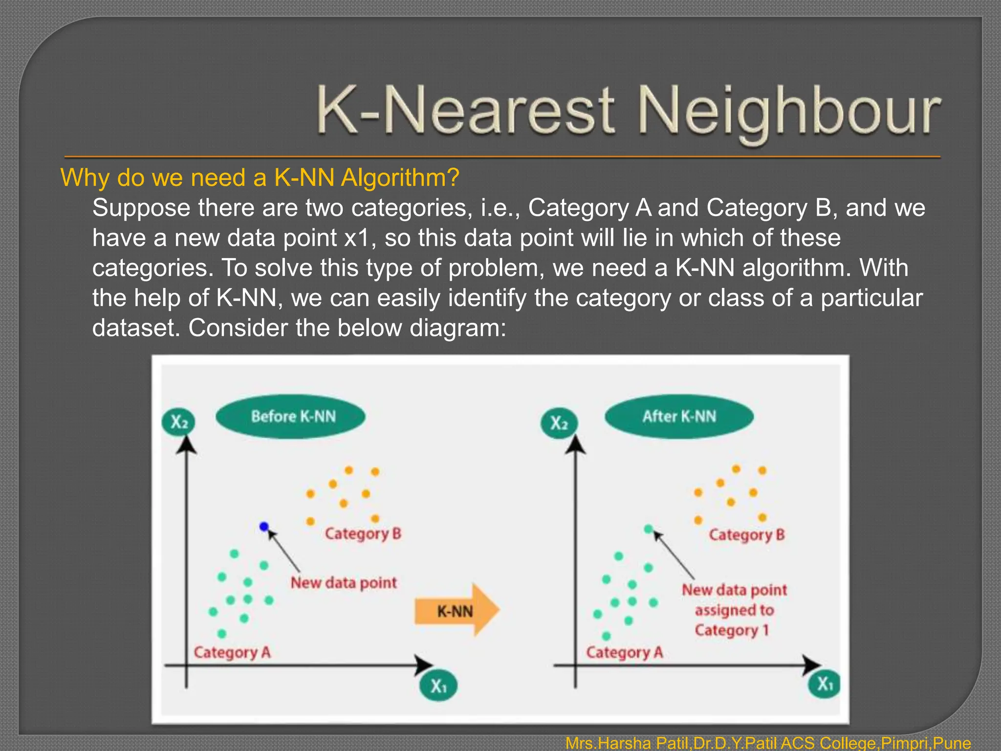
The document discusses classification algorithms, which are supervised machine learning techniques used to categorize new observations based on patterns learned from training data. Classification algorithms learn from labeled training data to classify future observations into a finite number of classes or categories. The document provides examples of classification including spam detection and categorizing images as cats or dogs. It describes key aspects of classification algorithms like binary and multi-class classification and discusses specific algorithms like logistic regression and support vector machines (SVM).
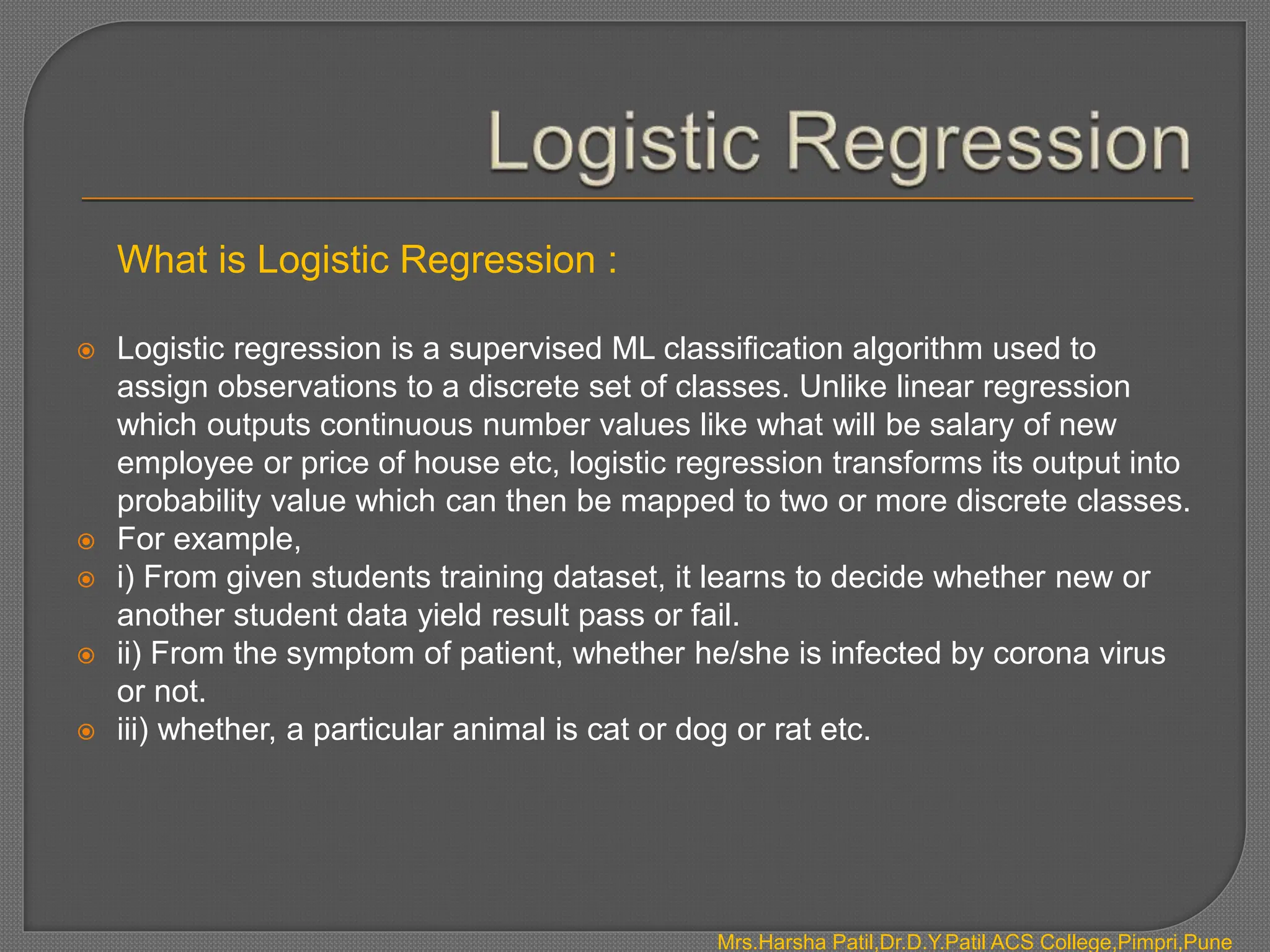
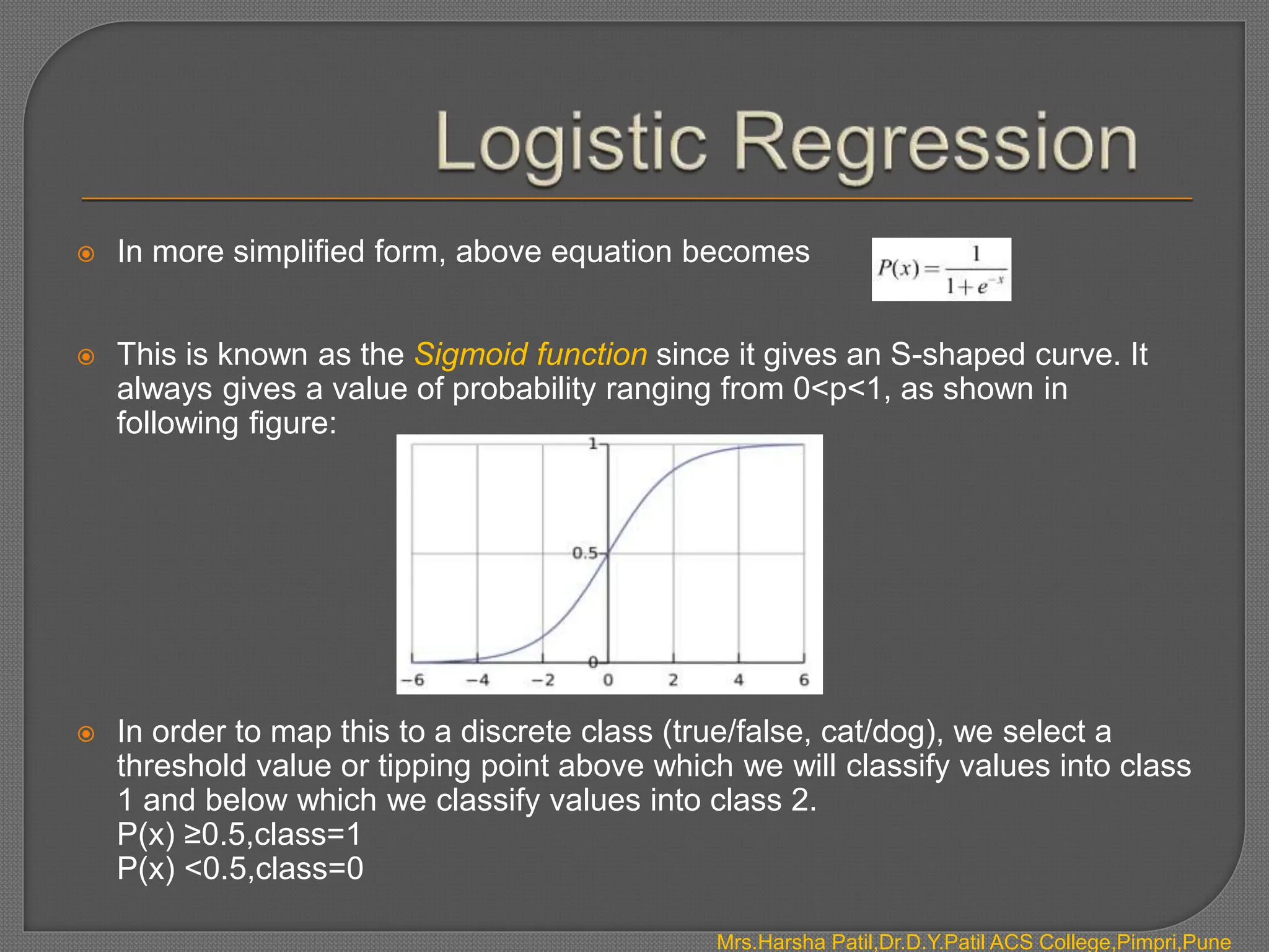
![ To avoid this problem, log-odds function or logit function is used.
Logistic regression can therefore be expressed in terms of logit function as :
log(P(x)/1-P(x)) = b0 + b1 * X
where, the left-hand side is called the logit or log-odds function, and p(x)/(1-
p(x)) is called odds.
The odds signify the ratio of probability of success [p(x)] to probability of failure [
1- p(X)]. Therefore, in Logistic Regression, linear combination of inputs is
mapped to the log(odds) - the output being equal to 1.
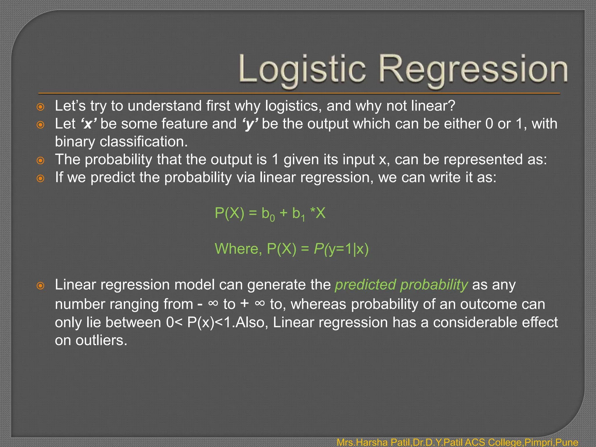
If we take an inverse of the above function, we get:
P(x) =
Mrs.Harsha Patil,Dr.D.Y.Patil ACS College,Pimpri,Pune](https://image.slidesharecdn.com/introductiontoclassification-240407070920-ae4b4e54/75/Introduction-to-Classification-pptx-11-2048.jpg)


![[DSC Europe 25] Jim Sterne - Adopting Generative AI Capabilities Into the Ent...](https://cdn.slidesharecdn.com/ss_thumbnails/sxhpofuorcagxsaulkmt-3-251204082258-7e66bc48-thumbnail.jpg?width=640&height=640&fit=bounds)


![[DSC Europe 25] Boris Perkovic - Lost in performance.pptx](https://cdn.slidesharecdn.com/ss_thumbnails/uq5hrp7vsuahqkxzifux-1-251204082258-fd2ee09d-thumbnail.jpg?width=640&height=640&fit=bounds)

![[DSC Europe 25] Dusan Jovicic - AI Story: From on-prem to cloud and back agai...](https://cdn.slidesharecdn.com/ss_thumbnails/8kp49m6uq22ifnbwhfnk-2-251205085715-964d11a6-thumbnail.jpg?width=640&height=640&fit=bounds)
![[DSC Europe 25] Marija Vlajkovic & Andrea Radonjanin - Integration of AI tool...](https://cdn.slidesharecdn.com/ss_thumbnails/qf1jrglttoc3bm8s3aop-final-integration-of-ai-tools-251208151905-394f3a6a-thumbnail.jpg?width=640&height=640&fit=bounds)
![[DSC Europe 25] Max Talanov - Non digital NNs.pptx](https://cdn.slidesharecdn.com/ss_thumbnails/wif8tr3gtua74qvtopke-non-digital-nns-251205090438-26b0eea6-thumbnail.jpg?width=640&height=640&fit=bounds)

![[DSC Europe 25] Dragan Vucic - Building the Learning Organization - How AI Tr...](https://cdn.slidesharecdn.com/ss_thumbnails/8brigo2sbu6qur6gxrra-7-251205085715-6ae07d24-thumbnail.jpg?width=640&height=640&fit=bounds)
![[DSC Europe 25] Petar Zivanov - AI meets documents From chatbots to AI-powere...](https://cdn.slidesharecdn.com/ss_thumbnails/xer2bb6nrdc8pdpev0pc-8-251204082258-7c2fa4a1-thumbnail.jpg?width=640&height=640&fit=bounds)

