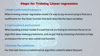
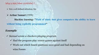
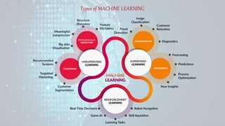
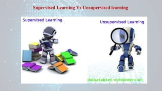
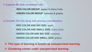
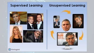
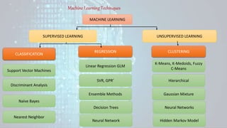
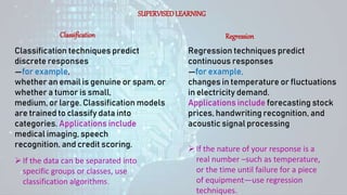
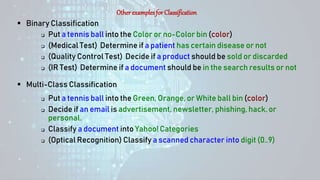
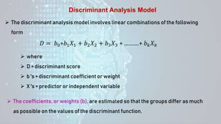
Machine Learning_PPT.pptx

What is MACHINE LEARNING ?....
 Not a well defined definition. But
 Arthur Samuel (1959):
Machine learning: "Field of study that gives computers the ability to learn
without being explicitly programmed"
 Samuel wrote a checkers playing program
 Had the program play 10000 games against itself
 Work out which board positions were good and bad depending on
wins/losses
Example

 Tom Michel (1999):
Well posed learning problem: "A computer program is said to learn from
experience E with respect to some class of tasks T and performance measure P, if
its performance at tasks in T, as measured by P, improves with experience E."
An other definition……
The checkers example,
 E = 10000s games
 T is playing checkers
 P if you win or loss

Is Machine Learning Magic?
No,
It is more like gardening.
Seeds = Algorithms
Nutrients = Data
Gardener = You
Plants = Programs

Supervised Learning (Train me)
 It is a data mining task of inferring a function from labeled training data.
 The training data consist of a set of training examples.
 In supervised learning, each example is a pair consisting of an input object (typically a
vector) and the desired output value (also called the supervisory signal)
Unsupervised Learning (I am self sufficient in learning)
 That learns from test data that has not been labeled, classified or categorized.
 Instead of responding to feedback, unsupervised learning identifies commonalities in
the data and reacts based on the presence or absence of such commonalities in each new
piece of data

Reinforcement Learning (My life My rules! (Hit & Trail))
 It is the ability of an agent to interact with the environment and find out what is the best
outcome. It follows the concept of hit and trial method.
 The agent is rewarded with a point for a correct or a wrong answer, and on the basis of
the positive reward points gained the model trains itself.
 Reinforcement learning differs from the supervised learning in a way that in supervised
learning, the training data has the answer key with it so the model is trained with the
correct answer itself whereas in reinforcement learning, there is no answer but the
reinforcement agent decides what to do to perform the given task
 In the absence of training dataset, it is bound to learn from its experience.

Supervised
Unsupervised
Learning
Reinforcemen
t
• Labeled data
• Direct feedback
• Predict outcome/future
• Decision Process
• Reward System
• Learn series of actions
• No labels
• No feedback
• Find hidden Structure

Supervised Learning Vs Unsupervised learning

Real Life example
Task is to arrange them as
groups
NO SIZE Colour Shape Fruit Name
1 Big Red
Rounded shape with a
depression at the top
Apple
2 Small Red
Heart-shaped to nearly
globular
Cherry
3 Big Green Long curving cylinder Banana
4 Small Green
Round to oval, Bunch
shape cylindrical
Grape

For Supervised Learning
 Already learn from previous work about the physical characters of fruits
 So arranging the same type of fruits at one place.
 Your previous work is called as training data in data mining
 You already learn the things from your train data, this is because of
response variable
 Response variable means just a decision variable

For Unsupervised Learning
 This time we don’t know any thing about the fruits, honestly saying this
is the first time you have seen them. You have no clue about those.
 So, how will we arrange them?
 What will we do first???
 We will take a fruit and you will arrange them by considering physical
character of that particular fruit.

 Suppose We have considered color
•RED COLOR GROUP: apples & cherry fruits.
•GREEN COLOR GROUP: bananas & grapes.
 Consider The Size along with previous consideration:
•RED COLOR AND BIG SIZE: apple.
•RED COLOR AND SMALL SIZE: cherry fruits.
•GREEN COLOR AND BIG SIZE: bananas.
•GREEN COLOR AND SMALL SIZE: grapes.
 This type of learning is known as unsupervised learning.
 Clustering comes under unsupervised learning.

Machine Learning Techniques
MACHINE LEARNING
SUPERVISED LEARNING UNSUPERVISED LEARNING
CLASSIFICATION
Nearest Neighbor
SVR, GPR’
Decision Trees
Neural Network
REGRESSION
Linear Regression GLM
Ensemble Methods
CLASSIFICATION
Support Vector Machines
Discriminant Analysis
Naïve Bayes
Hierarchical
Neural Networks
Hidden Markov Model
CLUSTERING
K-Means, K-Medoids, Fuzzy
C-Means
Gaussian Mixture

Selecting the Right Algorithm
 selecting a machine learning algorithm is a process of trial and error.
 It’s also a trade-off between specific characteristics of the algorithms,
such as:
 Speed of training
 Memory usage
 Predictive accuracy on new data
 Transparency or interpretability (how easily you can
understand the reasons an algorithm makes its predictions)

SUPERVISEDLEARNING
Classification Regression
Classification techniques predict
discrete responses
—for example,
whether an email is genuine or spam, or
whether a tumor is small,
medium, or large. Classification models
are trained to classify data into
categories. Applications include
medical imaging, speech
recognition, and credit scoring.
Regression techniques predict
continuous responses
—for example,
changes in temperature or fluctuations
in electricity demand.
Applications include forecasting stock
prices, handwriting recognition, and
acoustic signal processing
If the data can be separated into
specific groups or classes, use
classification algorithms.
If the nature of your response is a
real number –such as temperature,
or the time until failure for a piece
of equipment—use regression
techniques.

 Let’s take a closer look at the most commonly used
classification and regression algorithms.

Binaryvs. Multiclass Classification
When we are working on a classification problem, begin by determining whether
the problem is binary or multiclass.
BinaryClassification Multiclass Classification
A single training or test item (instance)
can only be divided into two classes
—for example, Determine whether an
email is genuine or spam
It can be divided into more than two
—for example, Train a model to classify
an image as a dog, cat, or other animal
It requires a more complex model

Binaryvs. Multiclass Classification
𝑋2
𝑋1
×
×
×
×
×
×
×
∆
∆
∆ ∆
∆
𝑋2
𝑋1
×
×
×
×
×
×
Binary Multiclass

Otherexamplesfor Classification
 Binary Classification
 Put a tennis ball into the Color or no-Color bin (color)
 (Medical Test) Determine if a patient has certain disease or not
 (Quality Control Test) Decide if a product should be sold or discarded
 (IR Test) Determine if a document should be in the search results or not
 Multi-Class Classification
 Put a tennis ball into the Green, Orange, or White ball bin (color)
 Decide if an email is advertisement, newsletter, phishing, hack, or
personal.
 Classify a document into Yahoo! Categories
 (Optical Recognition) Classify a scanned character into digit (0..9)

Support Vector Machine
 “Support Vector Machine” (SVM) is a supervised
machine learning algorithm which can be used
mostly in classification problems.
 In this algorithm, data plots as a points in n-
dimensional space (where n is number of
features) with the value of each feature being
the value of a particular coordinate.
 Then, classification perform by finding the
hyper-plane that differentiate the two classes
very well
hyper-plane

Margin
Margin
HowSupport vector machine Works
Classifies data by finding the linear decision boundary
(hyperplane) that separates all data points of one class
from those of the other class.
The best hyperplane for an SVM is the one with the
largest margin between the two classes, when the data is
linearly separable.
If the data is not linearly separable, a loss function is used
to penalize points on the wrong side of the hyperplane.
 SVMs sometimes use a kernel transform to transform nonlinearly separable data into
higher dimensions where a linear decision boundary can be found.

Identifythe right hyper-plane
 “Select the hyper-plane which segregates the two classes
better”.
 In this scenario, hyper-plane “B” has excellently performed
this job.
Which is the right hyper plane?
 Above, you can see that the margin for hyper-plane C is
high as compared to both A and B.
 Hence, we name the right hyper-plane as C.

Identifythe right hyper-plane
 SVM selects the hyper-plane which classifies the classes
accurately prior to maximizing margin.
 Here, hyper-plane B has a classification error and A has
classified all correctly.
 Therefore, the right hyper-plane is A.
 It solves this problem by introducing additional feature.
Here, we will add a new feature z=x^2+y^2. (Kernel
Transformation)
 Now, let’s plot the data points on axis x and z:

Support vector machine Best used ….
For data that has exactly two classes (you can also use it for multiclass classification with
a technique called error correcting output codes)
For high-dimensional, nonlinearly separable data

Pros and Cons associatedwithSVM
Pros:
 It works really well with clear margin of separation
 It is effective in high dimensionalspaces.
 It is effective in cases where number of dimensionsis greater than the number of samples.
 It uses a subset of training points in the decisionfunction (called support vectors), so it is also
memory efficient.
Cons:
 It doesn’t perform well, when we have large data set because the required training time is higher
 It also doesn’tperform very well, when the data set has more noise i.e. target classes are
overlapping
 SVM doesn’t directly provide probabilityestimates, these are calculated using an expensive five-fold
cross-validation.

Discriminant Analysis
Discriminant analysis (DA) is a technique for analyzing data when the criterion or
dependent variable is categorical and the predictor or independent variables are
interval in nature.
 It is a technique to discriminate between two or more mutually exclusive and
exhaustive groups on the basis of some explanatory variables
Types Discriminant Analysis (DA)
1. Linear D A - when the criterion /
dependent variable has two categories
Example: adopters & non-adopters
2. Multiple D A- when three or more
categories are involved
Example: SHG1, SHG2,SHG3

 Group sizes of the dependent should not be grossly different i.e. 80:20. It should be
at least five times the number of independent variables
How DA Works
Assumptions
1. Sample Size (n)
 Each of the independent variable is normally distributed.
2. Normal Distribution
 All variables have linear and homoscedastic relationships.
3. Homogeneity of variances / covariances

 Outliers should not be present in the data.
DA is highly sensitive to the inclusion of
outliers.
4. Outliers
 There should NOT BE MULTICOLLINEARITY
among the independent variables.
5. Non - multicolinearity

 The groups must be mutually exclusive, with every subject or case belonging to
only one group.
6. Mutually exclusive
 Each of the allocations for the dependent categories in the initial classification are
correctly classified.
7. Classification

Discriminant Analysis Model
 The discriminant analysis model involves linear combinations of the following
form
𝐷 = 𝑏0+𝑏1𝑋1 + 𝑏2𝑋2 + 𝑏3𝑋3 + ……….+ 𝑏𝑘𝑋𝑘
 where
 D = discriminant score
 b 's = discriminant coefficient or weight
 X 's = predictor or independent variable
 The coefficients, or weights (b), are estimated so that the groups differ as much
as possible on the values of the discriminant function.

Applications of Discriminant Analysis Model
 Discriminant analysis has been success fully used for many applications. As long
as we can transform the problem into a classification problem.
 DA can be used for original applications also
1. Identification
 TO identify type of customers that is likely to buy certain product in a store.
 Using simple questionnaires survey, we can get the features of customers
 DA will help to select which features can describe the group membership of
buy or not buy the product

3. Prediction
 Question “will it rain to day” can be thought as prediction.
 Prediction problem can be thought as assigning “today” to one of the two
possible groups of rain and dry
2. Decision Making
 Doctor diagnosing illness may be seen as which disease the patient has.
 This problem can be transform into classification problem by assigning the
patient to a number of possible groups of disease based on the Observation on
the symptoms

5. Learning
 Scientists want to teach robot to learn to talk can be seen as classification
problem.
 It assigns frequency , pitch, tune, and many other measurements of sound into
many groups of words
4. Pattern recognition
 To distinguish pedestrian from dogs and cars on capture image sequence of traffic
date is a classification problem

Naïve Bayes Model
 It is a classification technique based on Bayes theorem with an assumption of
independence among predictors.
 It is easy to build and particularly useful for very large datasets.
 It learns and predicts very fast and it does not require lots of storage.
 I has an Assumption : All features must be independent of each other
 It still returns very good accuracy in practice even when the independent
assumption does not hold

1. Real-time Prediction
Applications of Naïve Bayes Model
2. Multi - Class Prediction
3. Text Classification/ Spam Filtering/Sentiment Analysis
4. Recommendation System

Probability Basics
• Prior, conditional and joint probability for random variables
– Prior probability: P(x)
– Conditional probability: P(𝑥1|𝑥2), P(𝑥2|𝑥1)
– Relationship: P 𝑥1, 𝑥2 = 𝑃 𝑥2 𝑥1 𝑃 𝑥1 = 𝑃 𝑥1 𝑥2 𝑃 𝑥2
– Independence: )
(
)
(
)
),
(
)
|
(
),
(
)
|
( 2
1
2
1
2
1
2
1
2 x
P
x
P
,x
P(x
x
P
x
x
P
x
P
x
x
P 1 


)
(
)
(
)
(
)
(
x
x
x
P
c
P
c
|
P
|
c
P 
Discriminative Generative
Bayesian Rule

Event contains 2 boxes. Box 1 Contains 2 white balls and 3 red balls, Box 2
contains 4 white balls and 5 red balls. One ball is drawn at random from one of the
box and is found to be red. Find the probability that It was drawn from second
box.
Example to Understand Baye’s Theorem
Let Assume, Red ball = R, white ball = W, Box1 = A, Box2 = B
Probability for selected one as box1 P(A) =
1
2
Probability for selected box as box 2 P(B) =
1
2
Probability of getting red ball from box1 = P(R|A) =
3
5
Solution

With below tabulation of the 100 people, what is the conditional probability that a
certain member of the school is a ‘Teacher’ given that he is a ‘Man’?
Example to Understand Baye’s Theorem
Female Male Total
Teacher 8 12 20
Student 32 48 80
Total 40 60 100

The Naïve Bayes Model
 The Bayes Rule provides the formula for the probability of Y given X. But, in real-
world problems, you typically have multiple X variables
 When the features are independent, we can extend the Bayes Rule to what is
called Naive Bayes
 It is called ‘Naive’ because of the naive assumption that the X’s are independent
of each other.

Naive Bayes Example
 Say you have 1000 fruits which could be either ‘banana’, ‘orange’ or ‘other’. These
are the 3 possible classes of the Y variable.

For the sake of computing the probabilities, let’s aggregate the
training data to form a counts table like this.

Step1: Compute the ‘Prior’ probabilities for each of the class of
fruits.
P(Y=Banana) = 500 / 1000 = 0.50
P(Y=Orange) = 300 / 1000 = 0.30
P(Y=Other) = 200 / 1000 = 0.20.
Step 2: Compute the probability of evidence that goes in the
denominator..
P(x1=Long) = 500 / 1000 = 0.50
P(x2=Sweet) = 650 / 1000 = 0.65
P(x3=Yellow) = 800 / 1000 = 0.80

Step 3: Compute the probability of likelihood of evidences that goes
in the numerator..
P(x1=Long | Y=Banana) = 400 / 500 = 0.80
P(x2=Sweet | Y=Banana) = 350 / 500 = 0.70
P(x3=Yellow | Y=Banana) = 450 / 500 = 0.90
So, the overall probability of Likelihood of evidence for Banana =
0.8 * 0.7 * 0.9 = 0.504

Step 4: Substitute all the 3 equations into the Naive Bayes formula,
to get the probability that it is a banana.

Nearest Neighbor Algorithm
 Simple Analogy , Tell me about your friends (Who your neighbors are) , then I
will tell who you are

Other Names for Nearest neighbor Algorithm
 K-Nearest Neighbors
 Memory-Based Reasoning
 Example-Based Reasoning
 Instance-Based Learning
 Lazy Learning

What is KNN (K-Nearest Neighbor)
 A powerful classification algorithm used in pattern recognition.
 K nearest neighbors stores all available casesand classifies new
cases based on a similarity measure(e.g distance function)
 One of the top data mining algorithms used today.
 A non-parametric lazy learning algorithm (An Instancebased Learning
method).

When do we use KNN
 KNN can be used for both classification and regression predictive problems.
However, it is more widely used in classification problems in the industry.
 To evaluate any technique we generally look at 3 important aspects
 It is commonly used for its easy of interpretation and low calculation time.

How does KNN work?.....
KNN has the following basic steps:
1. Calculate distance
2. Find closest neighbors
3. Vote for labels

Training error rate and Validation error rate
.
 Segregate the training and validation from the initial dataset. then
 Plot the validation error curve to get the optimal value of K. This value of K
should be used for all predictions

Distance Measure for Continuous Variables
 Minkowski =

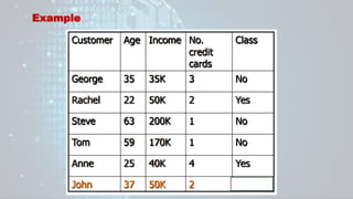
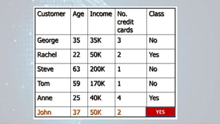
George to John Distance = Sqrt[(35 − 37)2+(35 − 50)2+(3 − 2)2] = 15.16
Rachel to John Distance = Sqrt[(22 − 37)2+(50 − 50)2+(2 − 2)2] = 15
Steve to John Distance = Sqrt[(63 − 37)2+(200 − 50)2+(1 − 2)2] = 152.23
Tom to John Distance = Sqrt[(59 − 37)2+(170 − 50)2+(1 − 2)2] = 122
Tom to John Distance = Sqrt[(25 − 37)2+(40 − 50)2+(4 − 2)2] = 15.74
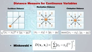
Distance Measure from john to others using Euclidean
Distance

Linear Regression
In regression problem the goal of the algorithm is to predict real-valued output.

Types of Regression
1. Simple Linear Regression
2. Polynomial Regression
3. Support Vector Regression
4. Decision Tree Regression
5. Random Forest Regression

Form of Linear Regression
𝑌 = 𝑏0+𝑏1𝑋1 + 𝑏2𝑋2 + 𝑏3𝑋3 + ……….+ 𝑏𝑘𝑋𝑘
 Y is the response
 b values are called the model coefficients. These values are “learned”
during the model fitting/training step.
 𝑏0 is the intercept
 𝑏1 is the coefficient for X1 (the first feature)
 𝑏𝑘 is the coefficient for Xn (the nth feature)

Steps for Training Linear regression
1. Model Coefficients/Parameters
When training a linear regression model it’s way to say we are trying to find out a
coefficients for the linear function that best describe the input variables.
2. Cost Function (Loss Function)
When building a linear model it’s said that we are trying to minimize the error an
algorithm does making predictions, and we got that by choosing a function to help
us measure the error also called cost function.
3.Estimate The Coefficients
For that task there’s a mathematical algorithm called Gradient Descent,

Model evaluation metrics for regression
 It is necessary to evaluate metrics designed for comparing continuous values
 Root Mean Squared Error, is on of the best evaluation methods
1
𝑛
𝑖=1
𝑛
(𝑦𝑖 − 𝑦𝑚𝑒𝑎𝑛)2

Learn More About machine learning through Online Courses
1. Coursera – Machine Learning- Andrew N.G. – Stanford University
2. Machine Learning for Intelligent Systems – Kilian Weinberger

Machine Learning_PPT.pptx

More Related Content

Similar to Machine Learning_PPT.pptx

Recently uploaded

Machine Learning_PPT.pptx