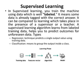
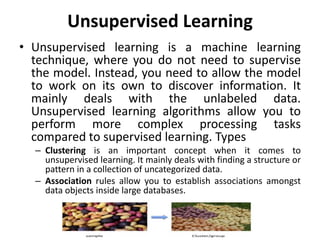
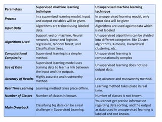
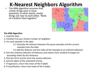
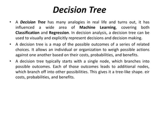
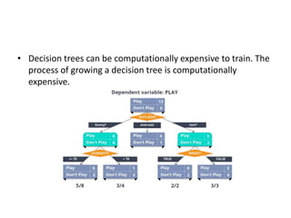
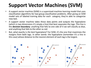
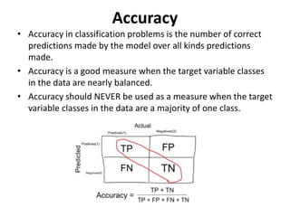
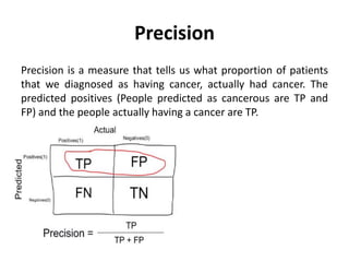
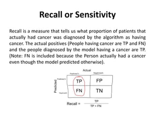
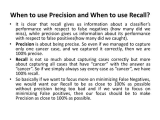
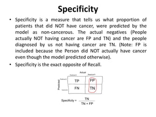
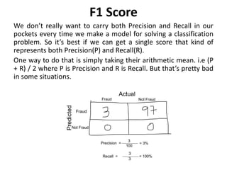
Supervised learning uses labeled training data to predict outcomes for new data. Unsupervised learning uses unlabeled data to discover patterns. Some key machine learning algorithms are described, including decision trees, naive Bayes classification, k-nearest neighbors, and support vector machines. Performance metrics for classification problems like accuracy, precision, recall, F1 score, and specificity are discussed.

1. Supervised & Unsupervised
Learning
~S. Amanpal

2. Supervised Learning
• In Supervised learning, you train the machine
using data which is well "labeled." It means some
data is already tagged with the correct answer. It
can be compared to learning which takes place in
the presence of a supervisor or a teacher. A
supervised learning algorithm learns from labeled
training data, helps you to predict outcomes for
unforeseen data. Types
– Regression: technique predicts a single output value using
training data.
– Classification: means to group the output inside a class.

3. Unsupervised Learning
• Unsupervised learning is a machine learning
technique, where you do not need to supervise
the model. Instead, you need to allow the model
to work on its own to discover information. It
mainly deals with the unlabeled data.
Unsupervised learning algorithms allow you to
perform more complex processing tasks
compared to supervised learning. Types
– Clustering is an important concept when it comes to
unsupervised learning. It mainly deals with finding a structure or
pattern in a collection of uncategorized data.
– Association rules allow you to establish associations amongst
data objects inside large databases.

4. Parameters
Supervised machine learning
technique
Unsupervised machine learning
technique
Process
In a supervised learning model, input
and output variables will be given.
In unsupervised learning model, only
input data will be given
Input Data
Algorithms are trained using labeled
data.
Algorithms are used against data which
is not labeled
Algorithms Used
Support vector machine, Neural
network, Linear and logistics
regression, random forest, and
Classification trees.
Unsupervised algorithms can be divided
into different categories: like Cluster
algorithms, K-means, Hierarchical
clustering, etc.
Computational
Complexity
Supervised learning is a simpler
method.
Unsupervised learning is
computationally complex
Use of Data
Supervised learning model uses
training data to learn a link between
the input and the outputs.
Unsupervised learning does not use
output data.
Accuracy of Results
Highly accurate and trustworthy
method.
Less accurate and trustworthy method.
Real Time Learning Learning method takes place offline.
Learning method takes place in real
time.
Number of Classes Number of classes is known. Number of classes is not known.
Main Drawback
Classifying big data can be a real
challenge in Supervised Learning.
You cannot get precise information
regarding data sorting, and the output
as data used in unsupervised learning is
labeled and not known.

5. Naive Bayes Classification
• It is a probabilistic classifier that makes classifications
using the Maximum A Posteriori decision rule in a
Bayesian setting.
• Bayes rule: P(A|B) = P(B|A) P(A) / P(B)
• where A and B are events
• Basically, we are trying to find probability of event A,
given the event B is true. Event B is also termed as
evidence.
• P(A) is the priori of A (the prior probability, i.e.
Probability of event before evidence is seen). The
evidence is an attribute value of an unknown
instance(here, it is event B).
• P(A|B) is a posteriori probability of B, i.e. probability of
event after evidence is seen.

6. – In the context of classification,
– you can replace A with a class, c_i, and
– B with our set of features, x_0 through x_n.
– Since P(B) serves as normalization
– P(c_i | x_0, …, x_n) ∝ P(x_0, …, x_n | c_i) * P(c_i)

7. • Now, if any two events A and B are independent,
then, P(A,B) = P(A)P(B) ; Hence:

8. Gaussian Naive Bayes classifier
In Gaussian Naive Bayes, continuous
values associated with each feature
are assumed to be distributed
according to a Gaussian distribution. A
Gaussian distribution is also called
Normal distribution. When plotted, it
gives a bell shaped curve which is
symmetric about the mean of the
feature values as shown below:
The likelihood of the features is assumed to be Gaussian, hence, conditional
probability is given by:

10. K-Nearest Neighbors Algorithm
• The KNN algorithm assumes that
similar things exist in close
proximity. In other words, similar
things are near to each other. “Birds
of a feather flock together.”
The KNN Algorithm
1. Load the data
2. Initialize K to your chosen number of neighbors
3. For each example in the data
3.1 Calculate the distance between the query example and the current
example from the data.
3.2 Add the distance and the index of the example to an ordered collection
4. Sort the ordered collection of distances and indices from smallest to largest (in
ascending order) by the distances
5. Pick the first K entries from the sorted collection
6. Get the labels of the selected K entries
7. If regression, return the mean of the K labels
8. If classification, return the mode of the K labels

11. Decision Tree
• A Decision Tree has many analogies in real life and turns out, it has
influenced a wide area of Machine Learning, covering both
Classification and Regression. In decision analysis, a decision tree can be
used to visually and explicitly represent decisions and decision making.
• A decision tree is a map of the possible outcomes of a series of related
choices. It allows an individual or organization to weigh possible actions
against one another based on their costs, probabilities, and benefits.
• A decision tree typically starts with a single node, which branches into
possible outcomes. Each of those outcomes leads to additional nodes,
which branch off into other possibilities. This gives it a tree-like shape. eir
costs, probabilities, and benefits.

12. • Decision trees can be computationally expensive to train. The
process of growing a decision tree is computationally
expensive.

13. Support Vector Machines (SVM)
• A support vector machine (SVM) is a supervised machine learning model that uses
classification algorithms for two-group classification problems. After giving an SVM
model sets of labeled training data for each category, they’re able to categorize
new text.
• A support vector machine takes these data points and outputs the hyperplane
(which in two dimensions it’s simply a line) that best separates the tags. This line is
the decision boundary: anything that falls to one side of it we will classify as blue,
and anything that falls to the other as red.
• But, what exactly is the best hyperplane? For SVM, it’s the one that maximizes the
margins from both tags. In other words: the hyperplane (remember it’s a line in
this case) whose distance to the nearest element of each tag is the largest.

14. • The points closest to the hyperplane are called as the support
vector points and the distance of the vectors from the
hyperplane are called the margins.

15. • Soft Margin SVM is better than Hard Margin SVM, because:
• Hard Margin SVM is quite sensitive to outliers.
• Soft Margin SVM avoids iterating over outliers.
• In the below diagram you can notice overfitting of hard
margin SVM.
• Soft-margin SVM can choose a decision boundary that has
non-zero training error even if the dataset is linearly
separable, and is less likely to overfit. You can notice that
decreasing C value causes the classifier to leave linear
separability in order to gain stability.

16. Support Vector Machines kernel
• The SVM model is a supervised machine learning model that is mainly
used for classifications (but it could also be used for regression!). It learns
how to separate different groups by forming decision boundaries.
• It sounds simple. However, not all data are linearly separable. In fact, in
the real world, almost all the data are randomly distributed, which makes
it hard to separate different classes linearly.

17. The kernel trick
• As you can see in the above picture, if we find a way to map the data from
2-dimensional space to 3-dimensional space, we will be able to find a
decision surface that clearly divides between different classes. My first
thought of this data transformation process is to map all the data point to
a higher dimension (in this case, 3 dimension), find the boundary, and
make the classification.
• That sounds alright. However, when there are more and more dimensions,
computations within that space become more and more expensive. This is
when the kernel trick comes in.
• It allows us to operate in the original feature space without computing the
coordinates of the data in a higher dimensional space.
• Let’s look at an example:

18. Here x and y are two data points in 3 dimensions. Let’s assume that we need
to map x and y to 9-dimensional space. We need to do the following
calculations to get the final result, which is just a scalar. The computational
complexity, in this case, is O(n²).
However, if we use the kernel function, which is denoted as k(x, y), instead of
doing the complicated computations in the 9-dimensional space, we reach the
same result within the 3-dimensional space by calculating the dot product of x -
transpose and y. The computational complexity, in this case, is O(n).

19. The kernel trick sounds like a “perfect” plan. However, one
critical thing to keep in mind is that when we map data to a
higher dimension, there are chances that we may overfit the
model. Thus choosing the right kernel function (including the
right parameters) and regularization are of great importance.

20. Performance Metrics for Classification
Confusion Matrix: The confusion matrix, is a table with two
dimensions (“Actual” and “Predicted”), and sets of “classes” in both
dimensions. Our Actual classifications are columns and Predicted
ones are Rows.
The Confusion matrix in itself is not a performance measure as such,
but almost all of the performance metrics are based on Confusion
Matrix and the numbers inside it.

21. Terms associated with Confusion matrix
Before diving into what the confusion matrix is all about and what it conveys, Let’s say we are solving a
classification problem where we are predicting whether a person is having cancer or not.
Let’s give a label of to our target variable:
1: When a person is having cancer 0: When a person is NOT having cancer.
• True Positives (TP): True positives are the cases when the actual class of the data point was 1(True)
and the predicted is also 1(True)
• Ex: The case where a person is actually having cancer(1) and the model classifying his case as
cancer(1) comes under True positive.
• 2. True Negatives (TN): True negatives are the cases when the actual class of the data point was
0(False) and the predicted is also 0(False
• Ex: The case where a person NOT having cancer and the model classifying his case as Not cancer
comes under True Negatives.
• 3. False Positives (FP): False positives are the cases when the actual class of the data point was
0(False) and the predicted is 1(True). False is because the model has predicted incorrectly and
positive because the class predicted was a positive one. (1)
• Ex: A person NOT having cancer and the model classifying his case as cancer comes under False
Positives.
• 4. False Negatives (FN): False negatives are the cases when the actual class of the data point was
1(True) and the predicted is 0(False). False is because the model has predicted incorrectly and
negative because the class predicted was a negative one. (0)
• Ex: A person having cancer and the model classifying his case as No-cancer comes under False
Negatives.

22. • The ideal scenario that we all want is that the
model should give 0 False Positives and 0 False
Negatives. But that’s not the case in real life as
any model will NOT be 100% accurate most of
the times.

23. Accuracy
• Accuracy in classification problems is the number of correct
predictions made by the model over all kinds predictions
made.
• Accuracy is a good measure when the target variable classes
in the data are nearly balanced.
• Accuracy should NEVER be used as a measure when the target
variable classes in the data are a majority of one class.

24. Precision
Precision is a measure that tells us what proportion of patients
that we diagnosed as having cancer, actually had cancer. The
predicted positives (People predicted as cancerous are TP and
FP) and the people actually having a cancer are TP.

25. Recall or Sensitivity
Recall is a measure that tells us what proportion of patients that
actually had cancer was diagnosed by the algorithm as having
cancer. The actual positives (People having cancer are TP and FN)
and the people diagnosed by the model having a cancer are TP.
(Note: FN is included because the Person actually had a cancer
even though the model predicted otherwise).

26. When to use Precision and When to use Recall?
• It is clear that recall gives us information about a classifier’s
performance with respect to false negatives (how many did we
miss), while precision gives us information about its performance
with respect to false positives(how many did we caught).
• Precision is about being precise. So even if we managed to capture
only one cancer case, and we captured it correctly, then we are
100% precise.
• Recall is not so much about capturing cases correctly but more
about capturing all cases that have “cancer” with the answer as
“cancer”. So if we simply always say every case as “cancer”, we have
100% recall.
• So basically if we want to focus more on minimizing False Negatives,
we would want our Recall to be as close to 100% as possible
without precision being too bad and if we want to focus on
minimizing False positives, then our focus should be to make
Precision as close to 100% as possible.

27. Specificity
• Specificity is a measure that tells us what proportion of
patients that did NOT have cancer, were predicted by the
model as non-cancerous. The actual negatives (People
actually NOT having cancer are FP and TN) and the people
diagnosed by us not having cancer are TN. (Note: FP is
included because the Person did NOT actually have cancer
even though the model predicted otherwise).
• Specificity is the exact opposite of Recall.

28. F1 Score
We don’t really want to carry both Precision and Recall in our
pockets every time we make a model for solving a classification
problem. So it’s best if we can get a single score that kind of
represents both Precision(P) and Recall(R).
One way to do that is simply taking their arithmetic mean. i.e (P
+ R) / 2 where P is Precision and R is Recall. But that’s pretty bad
in some situations.