This document describes an experiment in digital signal processing involving linear and circular convolution using discrete Fourier transform (DFT) and inverse discrete Fourier transform (IDFT) techniques. The experiment uses MATLAB to compute the convolution of sample input signals x and h in both the linear and circular cases. Output results are displayed showing the convolution outputs match those obtained using built-in MATLAB convolution functions. The document provides code examples and output plots to demonstrate linear and circular convolution computation in the frequency domain.

1. ECE324: DIGITAL SIGNAL PROCESSING LABORATORY
Practical No.:-05
Roll No.: B-54 Registration No.:11205816 Name:Shyamveer Singh
Program Codes: (Function files)
Circular Convolution:
Marks Obtained
Job Execution (Out of 40):_________
Online Submission (Out of 10):________
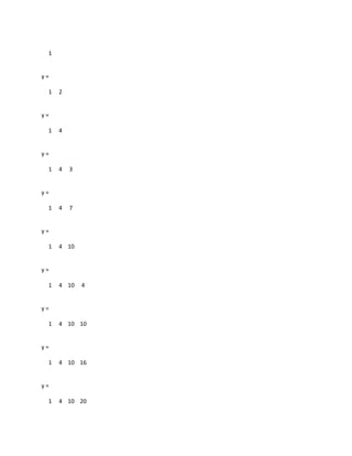
Aim: To compute the convolution linear and curricular both using DFT and IDFT techniques.
Mathematical Expressions Required:
Inputs (Should be allocated by the Instructor, Individually):
1. Linear Convolution
x=[1 2 3 4]
h=[1 2 3 4]
2. Circular Convolution
X=[1 2 3 4]
H=[1 2 3 4]
3. Circular Convolution
X=[1 2 3 4]
H=[1 2 3 4]

2. function[y]=shyamcconv(x,h)
m=length(x)
l=length(h)
n=m+l-1
for t=1:n
y(t)=0;
for k=max(1,t-(m-1)):min(t,m)
y(t)=y(t)+x(k).*h(mod(t-k+1,n))
end
end
z=y
y=cconv(x,h)
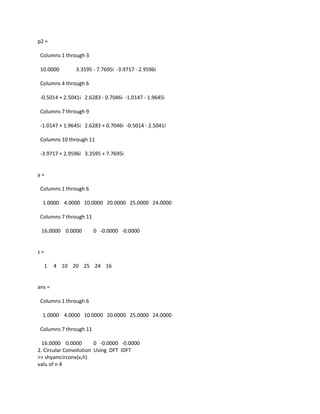
LINEAR CONVOLUTION USING DFT AND IDFT:
function[y]=shyamlinconv(x,h)
Nx=length(x)
Nh=length(h)
Ny=Nx+Nh-1
X=[x,zeros(1,Ny)]
H=[h,zeros(1,Ny)]
p1=fft(X)
p2=fft(H)
p=p1.*p2;
y=ifft(p)
z=conv(x,h)
end
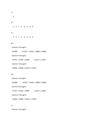
CIRCULAR CONVOLUTION USING DFT OR IDFT
function[y]=shyamcirconv(x,h)
n=input('valu of n')
X=[x,zeros(1,n)]
H=[h,zeros(1,n)]
p1=fft(X)
p2=fft(H)
p=p1.*p2;
y=ifft(p)
z=cconv(x,h)
end
Outputs/ Graphs/ Plots:
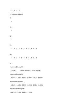
1. Linear Convolution :
>> x=[1 2 3 4]
x =
1 2 3 4
>> h=[1 2 3 4]
h =

3. 1 2 3 4
>> shyamlinconv(x,h)
Nx =
4
Nh =
4
Ny =
7
X =
1 2 3 4 0 0 0 0 0 0 0
H =
1 2 3 4 0 0 0 0 0 0 0
p1 =
Columns 1 through 3
10.0000 3.3595 - 7.7695i -3.9717 - 2.9596i
Columns 4 through 6
-0.5014 + 2.5041i 2.6283 - 0.7046i -1.0147 - 1.9645i
Columns 7 through 9
-1.0147 + 1.9645i 2.6283 + 0.7046i -0.5014 - 2.5041i
Columns 10 through 11
-3.9717 + 2.9596i 3.3595 + 7.7695i

4. p2 =
Columns 1 through 3
10.0000 3.3595 - 7.7695i -3.9717 - 2.9596i
Columns 4 through 6
-0.5014 + 2.5041i 2.6283 - 0.7046i -1.0147 - 1.9645i
Columns 7 through 9
-1.0147 + 1.9645i 2.6283 + 0.7046i -0.5014 - 2.5041i
Columns 10 through 11
-3.9717 + 2.9596i 3.3595 + 7.7695i
y =
Columns 1 through 6
1.0000 4.0000 10.0000 20.0000 25.0000 24.0000
Columns 7 through 11
16.0000 0.0000 0 -0.0000 -0.0000
z =
1 4 10 20 25 24 16
ans =
Columns 1 through 6
1.0000 4.0000 10.0000 20.0000 25.0000 24.0000
Columns 7 through 11
16.0000 0.0000 0 -0.0000 -0.0000
2. Circular Convolution Using DFT IDFT
>> shyamcirconv(x,h)
valu of n 4

5. n =
4
X =
1 2 3 4 0 0 0 0
H =
1 2 3 4 0 0 0 0
p1 =
Columns 1 through 3
10.0000 -0.4142 - 7.2426i -2.0000 + 2.0000i
Columns 4 through 6
2.4142 - 1.2426i -2.0000 2.4142 + 1.2426i
Columns 7 through 8
-2.0000 - 2.0000i -0.4142 + 7.2426i
p2 =
Columns 1 through 3
10.0000 -0.4142 - 7.2426i -2.0000 + 2.0000i
Columns 4 through 6
2.4142 - 1.2426i -2.0000 2.4142 + 1.2426i
Columns 7 through 8
-2.0000 - 2.0000i -0.4142 + 7.2426i
y =
Columns 1 through 6

6. 1.0000 4.0000 10.0000 20.0000 25.0000 24.0000
Columns 7 through 8
16.0000 -0.0000
z =
Columns 1 through 6
1.0000 4.0000 10.0000 20.0000 25.0000 24.0000
Column 7
16.0000
ans =
Columns 1 through 6
1.0000 4.0000 10.0000 20.0000 25.0000 24.0000
Columns 7 through 8
16.0000 -0.0000
2. Circular Convolution
>> shyamcconv(x,h)
m =
4
l =
4
n =
7
y =

7. 1
y =
1 2
y =
1 4
y =
1 4 3
y =
1 4 7
y =
1 4 10
y =
1 4 10 4
y =
1 4 10 10
y =
1 4 10 16
y =
1 4 10 20

8. y =
1 4 10 20 8
y =
1 4 10 20 17
y =
1 4 10 20 25
y =
1 4 10 20 25 12
y =
1 4 10 20 25 24
y =
1 4 10 20 25 24 16
z =
1 4 10 20 25 24 16
y =
Columns 1 through 6
1.0000 4.0000 10.0000 20.0000 25.0000 24.0000
Column 7
16.0000
ans =

9. Columns 1 through 6
1.0000 4.0000 10.0000 20.0000 25.0000 24.0000
Column 7
16.0000
Analysis/ Learning outcomes: After performing this experiment we know about the various
MATLAB commands and how to pad zeros in any signal and how to match the dimensions of
matrix.