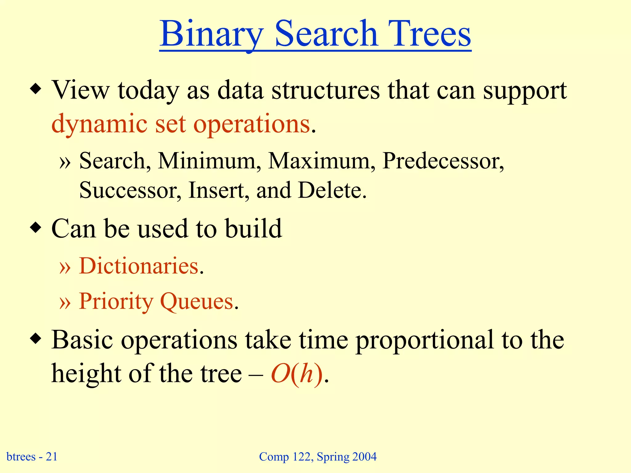
This document discusses binary search trees and red-black trees. It begins by defining binary search trees and describing their basic operations like search, insertion, and deletion which take time proportional to the height of the tree. It then introduces red-black trees, which add color attributes to nodes in a binary search tree to ensure the tree remains balanced, allowing operations to take O(log n) time. The properties of red-black trees are described, including that they guarantee all paths from a node to leaves contain the same number of black nodes.

1. Comp 122, Spring 2004
Binary Search Trees

2. btrees - 2 Comp 122, Spring 2004
Binary Trees
 Recursive definition
1. An empty tree is a binary tree
2. A node with two child subtrees is a binary tree
3. Only what you get from 1 by a finite number of
applications of 2 is a binary tree.
Is this a binary tree?
56
26 200
18 28 190 213
12 24 27

3. btrees - 3 Comp 122, Spring 2004
Binary Search Trees
 View today as data structures that can support
dynamic set operations.
» Search, Minimum, Maximum, Predecessor,
Successor, Insert, and Delete.
 Can be used to build
» Dictionaries.
» Priority Queues.
 Basic operations take time proportional to the
height of the tree – O(h).

4. btrees - 4 Comp 122, Spring 2004
BST – Representation
 Represented by a linked data structure of nodes.
 root(T) points to the root of tree T.
 Each node contains fields:
» key
» left – pointer to left child: root of left subtree.
» right – pointer to right child : root of right subtree.
» p – pointer to parent. p[root[T]] = NIL (optional).

5. btrees - 5 Comp 122, Spring 2004
Binary Search Tree Property
 Stored keys must satisfy
the binary search tree
property.
»  y in left subtree of x,
then key[y]  key[x].
»  y in right subtree of x,
then key[y]  key[x].
56
26 200
18 28 190 213
12 24 27

6. btrees - 6 Comp 122, Spring 2004
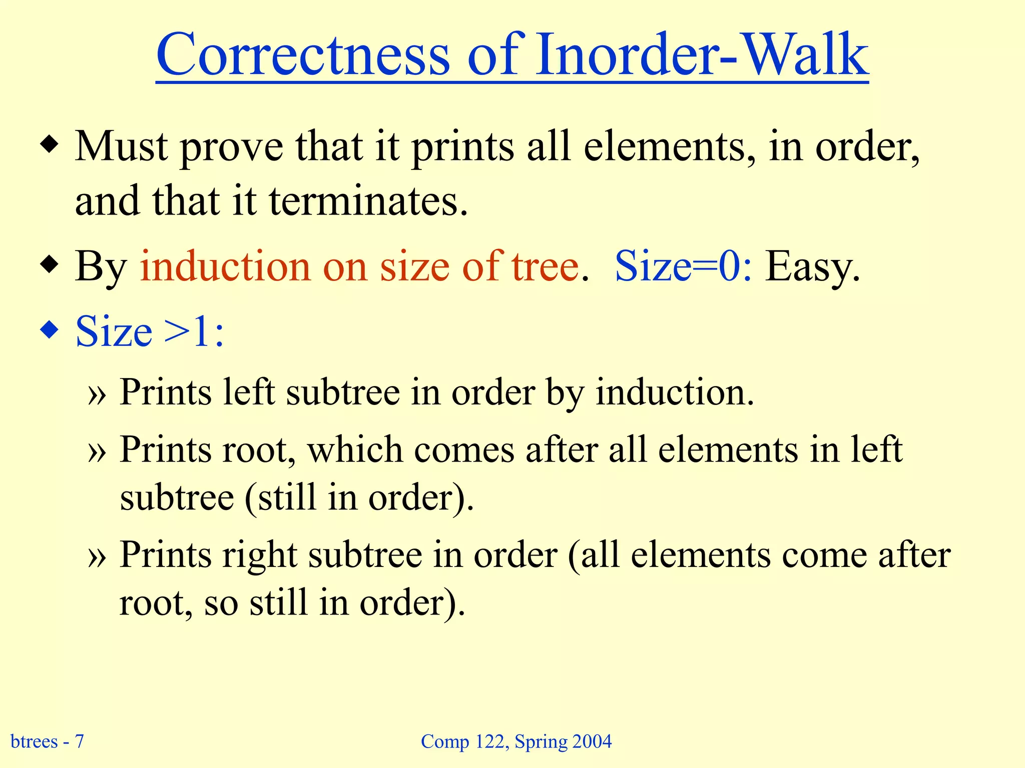
Inorder Traversal
Inorder-Tree-Walk (x)
1. if x  NIL
2. then Inorder-Tree-Walk(left[p])
3. print key[x]
4. Inorder-Tree-Walk(right[p])
 How long does the walk take?
 Can you prove its correctness?
The binary-search-tree property allows the keys of a binary search
tree to be printed, in (monotonically increasing) order, recursively.
56
26 200
18 28 190 213
12 24 27

7. btrees - 7 Comp 122, Spring 2004
Correctness of Inorder-Walk
 Must prove that it prints all elements, in order,
and that it terminates.
 By induction on size of tree. Size=0: Easy.
 Size >1:
» Prints left subtree in order by induction.
» Prints root, which comes after all elements in left
subtree (still in order).
» Prints right subtree in order (all elements come after
root, so still in order).

8. btrees - 8 Comp 122, Spring 2004
Querying a Binary Search Tree
 All dynamic-set search operations can be supported in
O(h) time.
 h = (lg n) for a balanced binary tree (and for an
average tree built by adding nodes in random order.)
 h = (n) for an unbalanced tree that resembles a linear
chain of n nodes in the worst case.

9. btrees - 9 Comp 122, Spring 2004
Tree Search
Tree-Search(x, k)
1. if x = NIL or k = key[x]
2. then return x
3. if k < key[x]
4. then return Tree-Search(left[x], k)
5. else return Tree-Search(right[x], k)
Running time: O(h)
Aside: tail-recursion
56
26 200
18 28 190 213
12 24 27

10. btrees - 10 Comp 122, Spring 2004
Iterative Tree Search
Iterative-Tree-Search(x, k)
1. while x  NIL and k  key[x]
2. do if k < key[x]
3. then x  left[x]
4. else x  right[x]
5. return x
The iterative tree search is more efficient on most computers.
The recursive tree search is more straightforward.
56
26 200
18 28 190 213
12 24 27

11. btrees - 11 Comp 122, Spring 2004
Finding Min & Max
Tree-Minimum(x) Tree-Maximum(x)
1. while left[x]  NIL 1. while right[x]  NIL
2. do x  left[x] 2. do x  right[x]
3. return x 3. return x
Q: How long do they take?
The binary-search-tree property guarantees that:
» The minimum is located at the left-most node.
» The maximum is located at the right-most node.

12. btrees - 12 Comp 122, Spring 2004
Predecessor and Successor
 Successor of node x is the node y such that key[y] is the
smallest key greater than key[x].
 The successor of the largest key is NIL.
 Search consists of two cases.
» If node x has a non-empty right subtree, then x’s successor is
the minimum in the right subtree of x.
» If node x has an empty right subtree, then:
• As long as we move to the left up the tree (move up through right
children), we are visiting smaller keys.
• x’s successor y is the node that x is the predecessor of (x is the maximum
in y’s left subtree).
• In other words, x’s successor y, is the lowest ancestor of x whose left
child is also an ancestor of x.

13. btrees - 13 Comp 122, Spring 2004
Pseudo-code for Successor
Tree-Successor(x)
 if right[x]  NIL
2. then return Tree-Minimum(right[x])
3. y  p[x]
4. while y  NIL and x = right[y]
5. do x  y
6. y  p[y]
7. return y
Code for predecessor is symmetric.
Running time: O(h)
56
26 200
18 28 190 213
12 24 27

14. btrees - 14 Comp 122, Spring 2004
BST Insertion – Pseudocode
Tree-Insert(T, z)
1. y  NIL
2. x  root[T]
3. while x  NIL
4. do y  x
5. if key[z] < key[x]
6. then x  left[x]
7. else x  right[x]
8. p[z]  y
9. if y = NIL
10. then root[t]  z
11. else if key[z] < key[y]
12. then left[y]  z
13. else right[y]  z
 Change the dynamic set
represented by a BST.
 Ensure the binary-
search-tree property
holds after change.
 Insertion is easier than
deletion.
56
26 200
18 28 190 213
12 24 27

15. btrees - 15 Comp 122, Spring 2004
Analysis of Insertion
 Initialization: O(1)
 While loop in lines 3-7
searches for place to
insert z, maintaining
parent y.
This takes O(h) time.
 Lines 8-13 insert the
value: O(1)
 TOTAL: O(h) time to
insert a node.
Tree-Insert(T, z)
1. y  NIL
2. x  root[T]
3. while x  NIL
4. do y  x
5. if key[z] < key[x]
6. then x  left[x]
7. else x  right[x]
8. p[z]  y
9. if y = NIL
10. then root[t]  z
11. else if key[z] < key[y]
12. then left[y]  z
13. else right[y]  z

16. btrees - 16 Comp 122, Spring 2004
Exercise: Sorting Using BSTs
Sort (A)
for i  1 to n
do tree-insert(A[i])
inorder-tree-walk(root)
» What are the worst case and best case running
times?
» In practice, how would this compare to other
sorting algorithms?

17. btrees - 17 Comp 122, Spring 2004
Tree-Delete (T, x)
if x has no children  case 0
then remove x
if x has one child  case 1
then make p[x] point to child
if x has two children (subtrees)  case 2
then swap x with its successor
perform case 0 or case 1 to delete it
 TOTAL: O(h) time to delete a node

18. btrees - 18 Comp 122, Spring 2004
Deletion – Pseudocode
Tree-Delete(T, z)
/* Determine which node to splice out: either z or z’s successor. */
 if left[z] = NIL or right[z] = NIL
 then y  z
 else y  Tree-Successor[z]
/* Set x to a non-NIL child of x, or to NIL if y has no children. */
4. if left[y]  NIL
5. then x  left[y]
6. else x  right[y]
/* y is removed from the tree by manipulating pointers of p[y]
and x */
7. if x  NIL
8. then p[x]  p[y]
/* Continued on next slide */

19. btrees - 19 Comp 122, Spring 2004
Deletion – Pseudocode
Tree-Delete(T, z) (Contd. from previous slide)
9. if p[y] = NIL
10. then root[T]  x
11. else if y  left[p[i]]
12. then left[p[y]]  x
13. else right[p[y]]  x
/* If z’s successor was spliced out, copy its data into z */
14. if y  z
15. then key[z]  key[y]
16. copy y’s satellite data into z.
17. return y

20. btrees - 20 Comp 122, Spring 2004
Correctness of Tree-Delete
 How do we know case 2 should go to case 0 or case
1 instead of back to case 2?
» Because when x has 2 children, its successor is the
minimum in its right subtree, and that successor
has no left child (hence 0 or 1 child).
 Equivalently, we could swap with predecessor
instead of successor. It might be good to alternate to
avoid creating lopsided tree.

21. btrees - 21 Comp 122, Spring 2004
Binary Search Trees
 View today as data structures that can support
dynamic set operations.
» Search, Minimum, Maximum, Predecessor,
Successor, Insert, and Delete.
 Can be used to build
» Dictionaries.
» Priority Queues.
 Basic operations take time proportional to the
height of the tree – O(h).

22. btrees - 22 Comp 122, Spring 2004
Red-black trees: Overview
 Red-black trees are a variation of binary search
trees to ensure that the tree is balanced.
» Height is O(lg n), where n is the number of nodes.
 Operations take O(lg n) time in the worst case.

23. btrees - 23 Comp 122, Spring 2004
Red-black Tree
 Binary search tree + 1 bit per node: the attribute
color, which is either red or black.
 All other attributes of BSTs are inherited:
» key, left, right, and p.
 All empty trees (leaves) are colored black.
» We use a single sentinel, nil, for all the leaves of
red-black tree T, with color[nil] = black.
» The root’s parent is also nil[T ].

24. btrees - 24 Comp 122, Spring 2004
Red-black Tree – Example
26
17
30 47
38 50
41
nil[T]

25. btrees - 25 Comp 122, Spring 2004
Red-black Properties
1. Every node is either red or black.
2. The root is black.
3. Every leaf (nil) is black.
4. If a node is red, then both its children are
black.
5. For each node, all paths from the node to
descendant leaves contain the same number of
black nodes.

26. btrees - 26 Comp 122, Spring 2004
Height of a Red-black Tree
 Height of a node:
» Number of edges in a longest path to a leaf.
 Black-height of a node x, bh(x):
» bh(x) is the number of black nodes (including nil[T ])
on the path from x to leaf, not counting x.
 Black-height of a red-black tree is the black-height
of its root.
» By Property 5, black height is well defined.

27. btrees - 27 Comp 122, Spring 2004
Height of a Red-black Tree
 Example:
 Height of a node:
» Number of edges in a
longest path to a leaf.
 Black-height of a node
bh(x) is the number of
black nodes on path from
x to leaf, not counting x.
26
17
30 47
38 50
41
nil[T]
h=4
bh=2
h=3
bh=2
h=2
bh=1
h=2
bh=1
h=1
bh=1
h=1
bh=1
h=1
bh=1

28. btrees - 28 Comp 122, Spring 2004
Hysteresis : or the value of lazyness
 Hysteresis, n. [fr. Gr. to be behind, to lag.]
a retardation of an effect when the forces acting
upon a body are changed (as if from viscosity or
internal friction); especially: a lagging in the
values of resulting magnetization in a magnetic
material (as iron) due to a changing magnetizing
force