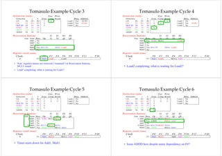
Instruction-level parallelism (ILP) aims to improve performance by overlapping the execution of instructions. There are two main approaches: 1) relying on hardware to dynamically discover and exploit parallelism, and 2) relying on software to statically find parallelism at compile-time. Exploiting ILP across multiple basic blocks is needed to achieve substantial performance gains, as basic block ILP is typically small due to frequent branches. Data dependencies between instructions limit the amount of parallelism that can be exploited, as true dependencies must be preserved to maintain program correctness. Hardware and software aim to exploit parallelism while preserving program order where it affects the program outcome.
![Outline
2.1 Instruction-Level Parallelism: Concepts and Challenges
Computer Architecture 2.2 Basic Compiler Techniques for Exposing ILP
計算機結構 2.3 Reducing Branch Costs with Prediction
2.4 Overcoming Data Hazards with Dynamic Scheduling
Lecture 3 2.5 Dynamic Scheduling: Examples and the Algorithm
Instruction-Level Parallelism 2.6
26 Hardware-Based Speculation
H d B dS l ti
2.7 Exploiting ILP Using Multiple Issue and Static Scheduling
and Its Exploitation
p 2.8
28 Exploiting ILP Using Dynamic Scheduling, Multiple Issue
Scheduling
(Chapter 2 in textbook) and Speculation
Ping-Liang Lai (賴秉樑)
Computer Architecture Ch3-1 Computer Architecture Ch3-2
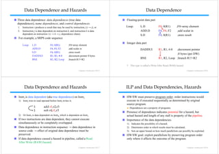
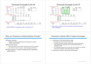
2.1 ILP: Concepts and Challenges Instruction-Level Parallelism (ILP)
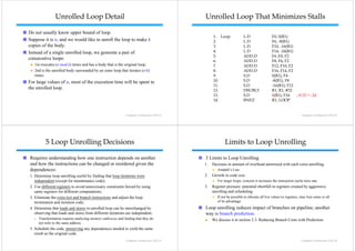
Instruction-Level Parallelism (ILP): overlap the execution of Basic Block (BB) ILP is quite small
instructions to improve performance. BB: a straight-line code sequence with no branches in except to the entry
2 approaches to exploit ILP and, no branches out except at the exit;
1) Rely on hardware to help discover and exploit the parallelism dynamically Average d
A dynamic branch frequency 15% to 25%;
i b hf t 25%
(e.g., Pentium 4, AMD Opteron, IBM Power), and » 3 to 6 instructions execute between a pair of branches.
2) Rely on software technology to find parallelism statically at compile-time
parallelism, Plus instructions in BB likely to depend on each other.
(e.g., Itanium 2) To obtain substantial performance enhancements, we must
Pipelining Review exploit ILP across multiple basic blocks. (ILP → LLP)
p p ( )
Pipeline CPI = Ideal pipeline CPI + Structural Stalls + Data Hazard Stalls Loop-Level Parallelism: to exploit parallelism among iterations of a loop.
+ Control Stalls E.g., add two matrixes.
for (i=1; i<=1000; i=i+1)
x[i] = x[i] + y[ ]
[] [ ] y[i];
Computer Architecture Ch3-3 Computer Architecture Ch3-4](https://image.slidesharecdn.com/chapter3instruction-levelparallelismanditsexploitation-130127203139-phpapp01/85/Chapter-3-instruction-level-parallelism-and-its-exploitation-1-320.jpg)
![Outline
2.1 Instruction-Level Parallelism: Concepts and Challenges
Computer Architecture 2.2 Basic Compiler Techniques for Exposing ILP
計算機結構 2.3 Reducing Branch Costs with Prediction
2.4 Overcoming Data Hazards with Dynamic Scheduling
Lecture 3 2.5 Dynamic Scheduling: Examples and the Algorithm
Instruction-Level Parallelism 2.6
26 Hardware-Based Speculation
H d B dS l ti
2.7 Exploiting ILP Using Multiple Issue and Static Scheduling
and Its Exploitation
p 2.8
28 Exploiting ILP Using Dynamic Scheduling, Multiple Issue
Scheduling
(Chapter 2 in textbook) and Speculation
Ping-Liang Lai (賴秉樑)
Computer Architecture Ch3-1 Computer Architecture Ch3-2
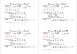
2.1 ILP: Concepts and Challenges Instruction-Level Parallelism (ILP)
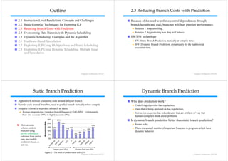
Instruction-Level Parallelism (ILP): overlap the execution of Basic Block (BB) ILP is quite small
instructions to improve performance. BB: a straight-line code sequence with no branches in except to the entry
2 approaches to exploit ILP and, no branches out except at the exit;
1) Rely on hardware to help discover and exploit the parallelism dynamically Average d
A dynamic branch frequency 15% to 25%;
i b hf t 25%
(e.g., Pentium 4, AMD Opteron, IBM Power), and » 3 to 6 instructions execute between a pair of branches.
2) Rely on software technology to find parallelism statically at compile-time
parallelism, Plus instructions in BB likely to depend on each other.
(e.g., Itanium 2) To obtain substantial performance enhancements, we must
Pipelining Review exploit ILP across multiple basic blocks. (ILP → LLP)
p p ( )
Pipeline CPI = Ideal pipeline CPI + Structural Stalls + Data Hazard Stalls Loop-Level Parallelism: to exploit parallelism among iterations of a loop.
+ Control Stalls E.g., add two matrixes.
for (i=1; i<=1000; i=i+1)
x[i] = x[i] + y[ ]
[] [ ] y[i];
Computer Architecture Ch3-3 Computer Architecture Ch3-4](https://image.slidesharecdn.com/chapter3instruction-levelparallelismanditsexploitation-130127203139-phpapp01/75/Chapter-3-instruction-level-parallelism-and-its-exploitation-1-2048.jpg)
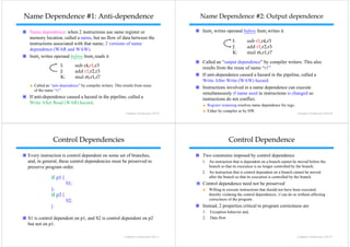
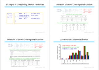
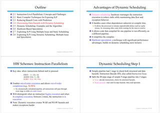
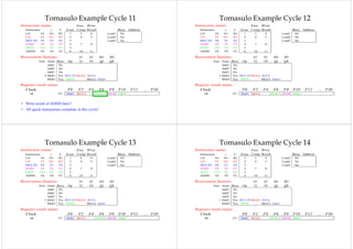
![Exception Behavior Data Flow
Preserving exception behavior Data flow: actual flow of data values among instructions that
Any changes in instruction execution order must not change how produce results and those that consume them.
exceptions are raised in program (⇒ no new exceptions). Branches make flow dynamic, determine which instruction is supplier of
Example
E l data.
data
Example
DADDU R2,R3,R4
BEQZ R2,L1 DADDU R1, R2, R3
LW R1,0(R2) BEQZ R4, L
L1: DSUBU R1 R5 R6
R1, R5,
L: …
† Assume branches not delayed. OR R7, R1, R8
Problem with moving LW before BEQZ? R1 of OR depends on DADDU or DSUBU?
Must preserve data flow on execution.
execution
Computer Architecture Ch3-13 Computer Architecture Ch3-14
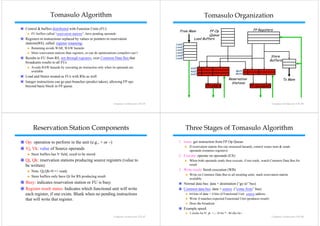
2.2 Basic Compiler Techniques
Outline for Exposing ILP
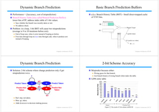
2.1 Instruction-Level Parallelism: Concepts and Challenges This code, add a scalar to a vector
2.2 Basic Compiler Techniques for Exposing ILP for (i=1000; i>0; i=i–1)
2.3 Reducing Branch Costs with Prediction x[i] = x[i] + s;
2.4 Overcoming Data Hazards with Dynamic Scheduling
Assume following latencies for all examples
2.5 Dynamic Scheduling: Examples and the Algorithm Ignore delayed branch in these examples
2.6
26 Hardware-Based Speculation
H d B dS l ti
2.7 Exploiting ILP Using Multiple Issue and Static Scheduling
Instruction producing result Instruction using result Latency in cycles
2.8
28 Exploiting ILP Using Dynamic Scheduling, Multiple Issue
Scheduling FP ALU op Another FP ALU op 3
and Speculation
FP ALU op Store double 2
Load d bl
L d double FP ALU op 1
Load double Store double 0
Figure 2.2 Latencies of FP operations used in this chapter.
Computer Architecture Ch3-15 Computer Architecture Ch3-16](https://image.slidesharecdn.com/chapter3instruction-levelparallelismanditsexploitation-130127203139-phpapp01/85/Chapter-3-instruction-level-parallelism-and-its-exploitation-4-320.jpg)


![[Harvard CS264] 02 - Parallel Thinking, Architecture, Theory & Patterns](https://cdn.slidesharecdn.com/ss_thumbnails/cs264201102-archtheorypatternshare-110206154047-phpapp02-thumbnail.jpg?width=640&height=640&fit=bounds)