Instruction level parallelism and techniques used for its implementations are discussed in this presentation

1. Advanced Techniques
For Exploiting ILP
Mr. A. B. Shinde
Assistant Professor,
Electronics Engineering,
P.V.P.I.T., Budhgaon

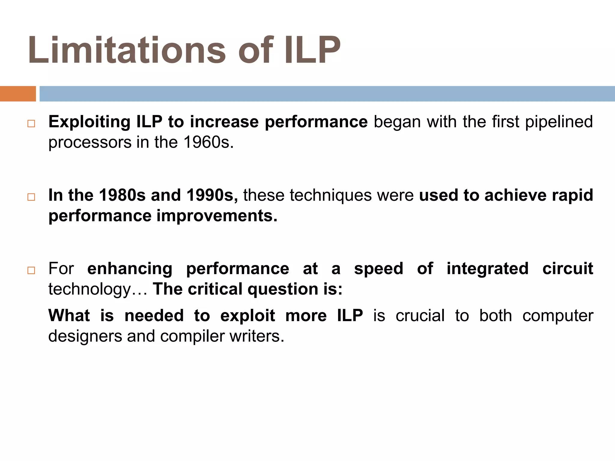
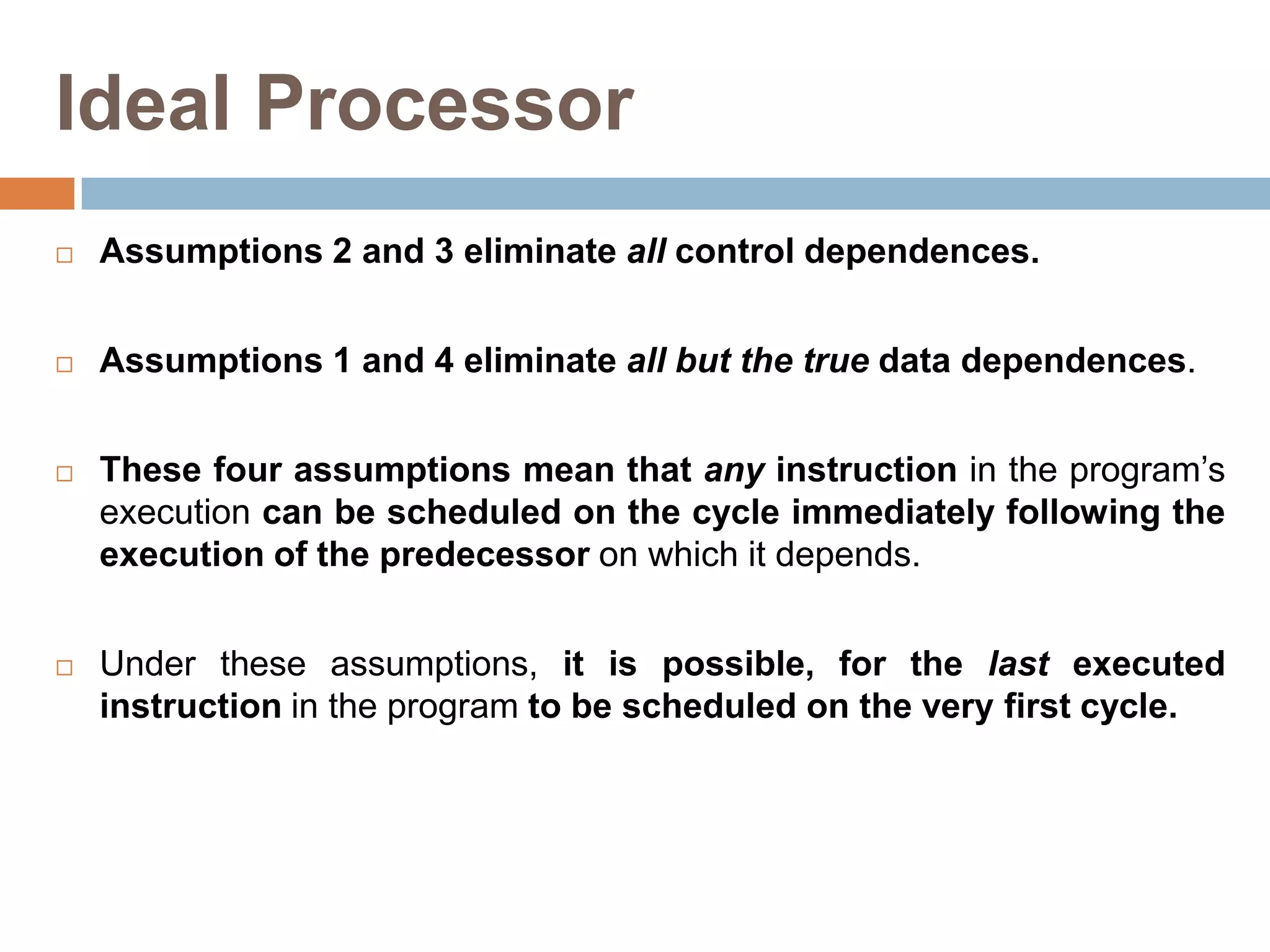
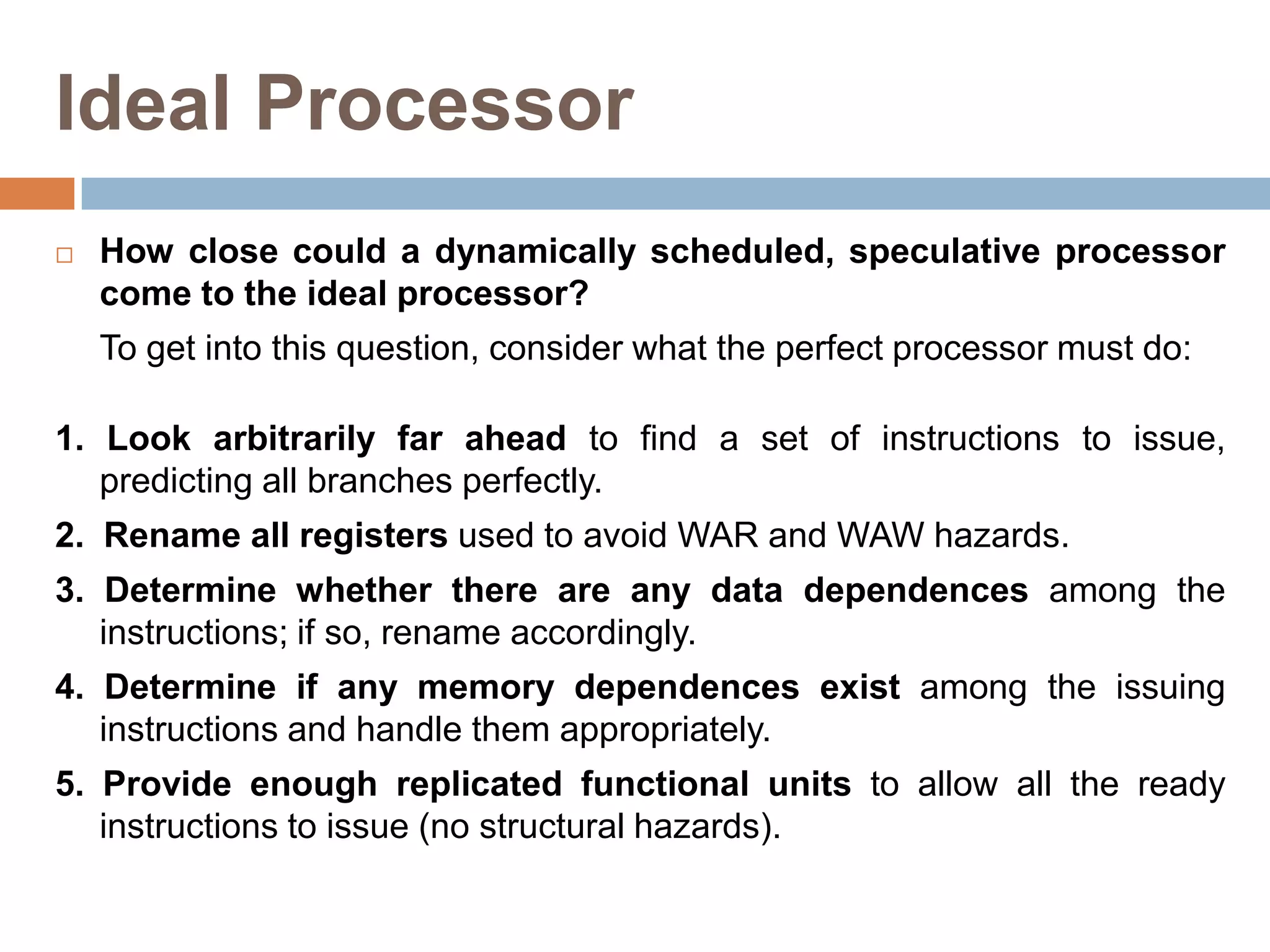
2. Contents…
 Complier techniques for
exposing ILP
 Limitation on ILP for realizable
Processors
 Hardware versus software
speculation
2

3. Pipelining
 Pipeline is a set of data processing elements connected in
series, so that the output of one element is the input of the next one.
 The elements of a pipeline are often executed in parallel.

4. Parallel Computing
 Parallel computing is a form of computation in which many
calculations are carried out simultaneously ("in parallel").
 There are several different forms of parallel computing:
 Bit-level,
 Instruction level,
 Data, and
 Task parallelism.

5. Instruction Level Parallelism (ILP)
 A computer program is, a stream of instructions executed by
a processor.
 These instructions can be re-ordered and combined into groups
which are then executed in parallel without changing the result of the
program.

6. Instruction Level Parallelism (ILP)
In ordinary programs instructions are executed in the order specified by
the programmer.
 How much ILP exists in programs is very application specific.
In certain fields, such as graphics and scientific computing the
amount can be very large.
However, workloads such as cryptography exhibit much less
parallelism.

7. Pipeline Scheduling
 The straightforward MIPS code, not scheduled for the pipeline, looks
like this:
Loop: L.D F0,0(R1) ;F0=array element
ADD.D F4,F0,F2 ;add scalar in F2
S.D F4,0(R1) ;store result
DADDUI R1,R1,#-8 ;decrement pointer by
;8 bytes
BNE R1,R2,Loop ;branch R1!=R2
 Let’s see how well this loop will run when it is scheduled on a simple
pipeline for MIPS.

8. Pipeline Scheduling
 Example: Show how the loop would look on MIPS, both scheduled and
unscheduled, including any stalls or idle clock cycles.
 Answer: Without any scheduling, the loop will execute as follows,
taking 9 cycles:
Clock cycle issued
Loop: L.D F0,0(R1) 1
stall 2
ADD.D F4,F0,F2 3
stall 4
stall 5
S.D F4,0(R1) 6
DADDUI R1,R1,#-8 7
stall 8
BNE R1,R2,Loop 9

9. Pipeline Scheduling
 We can schedule the loop to obtain only two stalls and reduce the
time to 7 cycles:
Clock cycles
Loop: L.D F0,0(R1) 1
DADDUI R1,R1,#-8 2
ADD.D F4,F0,F2 3
Stall 4
Stall 5
S.D F4,8(R1) 6
BNE R1,R2,Loop 7
 The stalls after ADD.D are for use by the S.D.
Clock cycles
Loop: L.D F0,0(R1) 1
stall 2
ADD.D F4,F0,F2 3
stall 4
stall 5
S.D F4,0(R1) 6
DADDUI R1,R1,#-8 7
stall 8
BNE R1,R2,Loop 9

10. Loop Unrolling
 In the previous example, we complete one loop iteration and store
back one array element every 7 clock cycles…
but the actual work of operating on the array element takes
just 3 (the load, add, and store) of those 7 clock cycles.
 The remaining 4 clock cycles consist of loop overhead—the
DADDUI and BNE—and two stalls.
 To eliminate these 4 clock cycles we need to get more operations
relative to the number of overhead instructions.
 A simple scheme for increasing the number of instructions relative to
the branch and overhead instructions is loop unrolling.
 Unrolling simply replicates the loop body multiple times.

11. Loop Unrolling
Loop: L.D F0,0(R1)
ADD.D F4,F0,F2
S.D F4,0(R1) ;drop DADDUI & BNE
L.D F6,-8(R1)
ADD.D F8,F6,F2
S.D F8,-8(R1) ;drop DADDUI & BNE
L.D F10,-16(R1)
ADD.D F12,F10,F2
S.D F12,-16(R1) ;drop DADDUI & BNE
L.D F14,-24(R1)
ADD.D F16,F14,F2
S.D F16,-24(R1)
DADDUI R1,R1,#-32
BNE R1,R2,Loop
Loop: L.D F0,0(R1)
DADDUI R1,R1,#-8
ADD.D F4,F0,F2
Stall
Stall
S.D F4,8(R1)
BNE R1,R2,Loop
Code without Loop unrolling
Code with Loop unrolling

12. Loop Unrolling
 Loop unrolling can also be used to improve scheduling, because it
eliminates the branch, it allows instructions from different iterations to be
scheduled together.
 If we simply replicated the instructions when we unrolled the loop,
the resulting use of the same registers could prevent us from
effectively scheduling the loop.
 Thus, the required number of registers will be increased.

13. Loop Unrolling and Scheduling:
Summary
 To obtain the final unrolled code we need to make the following
decisions and transformations:
 Determine that unrolling the loop would be useful by finding that the
loop iterations were independent.
 Use different registers to avoid unnecessary forcing by using the
same registers for different computations.
 Eliminate the extra test and branch instructions and adjust the loop
termination.
 Determine that the loads and stores in the unrolled loop can be
interchanged, if loads and stores from different iterations are
independent.
 Schedule the code, preserving any dependences needed to produce
same result as the original code.

14. Loop Unrolling and Scheduling:
Summary
 There are three different types of limits to the gains that can be
achieved by loop unrolling:
1. A decrease in the amount of overhead with each unroll,
2. Code size limitations, and
3. Compiler limitations.
Let’s consider the question of loop overhead first.
When we unrolled the loop four times, it generated sufficient
parallelism among the instructions that the loop could be scheduled
with no stall cycles.
In previous example, in 14 clock cycles, only 2 cycles were loop
overhead: the DADDUI, and BNE.

15. Loop Unrolling and Scheduling:
Summary
 A second limit to unrolling is the growth in code size.
 Factor often more important than code size is the potential shortfall
in registers that is created by aggressive unrolling and scheduling.
 The transformed code, is theoretically faster but it generates a
shortage of registers.

16. Loop Unrolling and Scheduling:
Summary
 Loop unrolling is a simple but useful method for increasing the size
of straight-line code fragments that can be scheduled effectively.
 This transformation is useful in a variety of processors, from simple
pipelines to the multiple-issue processors

17. Limitations of ILP

18. Limitations of ILP
 Exploiting ILP to increase performance began with the first pipelined
processors in the 1960s.
 In the 1980s and 1990s, these techniques were used to achieve rapid
performance improvements.
 For enhancing performance at a speed of integrated circuit
technology… The critical question is:
What is needed to exploit more ILP is crucial to both computer
designers and compiler writers.

19. Limitations of ILP
 To know what actually limits ILP…
… we first need to define an ideal processor.
 An ideal processor is one where all constraints on ILP are
removed.
 The only limits on ILP in ideal processor are by the actual data flows
through either registers or memory.

20. Ideal Processor
 The assumptions made for an ideal or perfect processor are as
follows:
1. Register renaming
There are an infinite number of virtual registers available, and hence
all WAW and WAR hazards are avoided and number of instructions
can begin execution simultaneously.
2. Branch prediction
Branch prediction is perfect. All conditional branches are predicted
exactly.
3. Jump prediction
All jumps are perfectly predicted.

21. Ideal Processor
 The assumptions made for an ideal or perfect processor are as
follows:
4. Memory address analysis
All memory addresses are known exactly, and a load can be moved
before a store provided that the addresses are not identical.
This implements perfect address analysis.
5. Perfect caches
All memory accesses take 1 clock cycle.

22. Ideal Processor
 Assumptions 2 and 3 eliminate all control dependences.
 Assumptions 1 and 4 eliminate all but the true data dependences.
 These four assumptions mean that any instruction in the program’s
execution can be scheduled on the cycle immediately following the
execution of the predecessor on which it depends.
 Under these assumptions, it is possible, for the last executed
instruction in the program to be scheduled on the very first cycle.

23. Ideal Processor
 How close could a dynamically scheduled, speculative processor
come to the ideal processor?
To get into this question, consider what the perfect processor must do:
1. Look arbitrarily far ahead to find a set of instructions to issue,
predicting all branches perfectly.
2. Rename all registers used to avoid WAR and WAW hazards.
3. Determine whether there are any data dependences among the
instructions; if so, rename accordingly.
4. Determine if any memory dependences exist among the issuing
instructions and handle them appropriately.
5. Provide enough replicated functional units to allow all the ready
instructions to issue (no structural hazards).

24. Ideal Processor
 For example, to determine whether n issuing instructions have any
register dependences among them, assuming all instructions are
register-register and the total number of registers is unbounded,
requires
Thus, issuing only 50 instructions requires 2450 comparisons.
This cost obviously limits the number of instructions that can be
considered for issue at once.
comparisons.

25. Limitations on ILP for Realizable
Processors
 The limitations are divided into two classes:
 Limitations that arise even for the perfect speculative processor,
and
 Limitations that arise for one or more realistic models.

26. Limitations on ILP for Realizable
Processors
 The most important limitations that apply even to the perfect model are
1. WAW and WAR hazards through memory
The WAW and WAR hazards are eliminated through register
renaming, but not in memory usage.
A normal procedure reuses the memory locations of a previous
procedure on the stack, and this can lead to WAW and WAR hazards.

27. Limitations on ILP for Realizable
Processors
 The most important limitations that apply even to the perfect model are
2. Unnecessary dependences
With infinite numbers of registers, all but true register data
dependences are removed.
There are, dependences arising from either recurrences or code
generation conventions that introduce unnecessary data dependences.
Code generation conventions introduce unneeded dependences, in
particular the use of return address registers and a register for the stack
pointer (which is incremented and decremented in the call/return
sequence).

28. Limitations on ILP for Realizable
Processors
 The most important limitations that apply even to the perfect model are
3. Overcoming the data flow limit
If value prediction worked with high accuracy, it could overcome the
data flow limit.
It is difficult to achieve significant enhancement in ILP, using a prediction
scheme.

29. Limitations on ILP for Realizable
Processors
 For a less-than-perfect processor, several ideas have been
proposed that could expose more ILP.
 To speculate along multiple paths: This idea was discussed by Lam
and Wilson [1992]. By speculating on multiple paths, the cost of
incorrect recovery is reduced and more parallelism can be
exposed.
 Wall [1993] provides data for speculating in both directions on up to
eight branches.
Out of both paths, one will be thrown away.
Every commercial design has instead devoted additional hardware to
better speculation on the correct path.

30. Hardware Vs Software Speculation

31. Hardware Vs Software Speculation
 To speculate extensively, we must be able to disambiguate (clear
the ambiguity) memory references.
 This capability is difficult to do at compile time for integer
programs that contain pointers.
 In a hardware-based scheme, dynamic run time disambiguation of
memory addresses is done using Tomasulo’s algorithm.

32. Hardware Vs Software Speculation
 Hardware-based speculation works better when control flow is
unpredictable, and
Hardware-based branch prediction is superior than software-based
branch prediction done at compile time.
For example:
a good static predictor has a misprediction rate of about 16% for four
major integer SPEC92 programs, and a hardware predictor has a
misprediction rate of under 10%, because, speculated instructions may
slow down the computation when the prediction is incorrect.

33. Hardware Vs Software Speculation
 Hardware-based speculation maintains a completely precise
exception model even for speculated instructions.
 Hardware-based speculation does not require compensation or
book-keeping code, which is needed by software speculation
mechanisms.
 Compiler-based approaches may benefit from the ability to see
further in the code sequence, resulting in better code scheduling than
a purely hardware driven approach.

34. Hardware Vs Software Speculation
 Hardware-based speculation with dynamic scheduling does not
require different code sequences to achieve good performance for
different implementations of an architecture.
 On the other hand, more recent explicitly parallel architectures,
(such as IA-64), have added flexibility that reduces the hardware
dependence inherent in a code sequence.

35. Hardware Vs Software Speculation
 The major disadvantage of supporting speculation in hardware is
the complexity and additional hardware resources required.
 Some designers have tried to combine the dynamic and compiler-based
approaches to achieve the best of each.
 For example:
If conditional moves are combined with register renaming, then a slight
side effect appears. A conditional move that is invalid must copy a value
to the destination register, since it was renamed earlier.

36. Thank You…
shindesir.pvp@gmail.com
(This Presentation is Published Only for Educational Purpose)