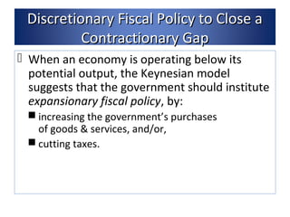
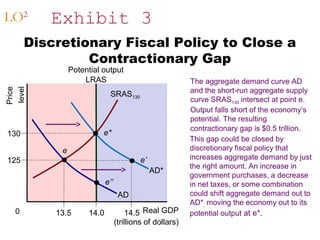
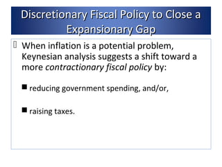
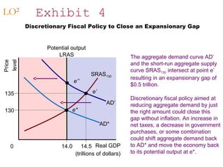
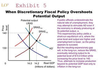
Chapter 11 
FFiissccaall PPoolliiccyy
TThheeoorryy ooff FFiissccaall PPoolliiccyy 
 What is fiscal policy? 
 Government purchases, transfer payments, taxes, 
and borrowing as they affect macroeconomic 
variables such as real GDP, employment, the price 
level, and economic growth.
FFiissccaall PPoolliiccyy TToooollss 
 Two categories: 
 Automatic stabilizers 
 Automatic stabilizers are revenue and spending programs in 
the federal budget that automatically adjust with the ups 
and downs of the economy to stabilize disposable income 
and, consequently, consumption and real GDP. 
 Example: Federal income tax 
 Discretionary fiscal policy 
 Requires the deliberate manipulation of government 
purchases, transfer payments, and taxes to promote 
macroeconomic goals.
DDiissccrreettiioonnaarryy FFiissccaall PPoolliiccyy 
 Increases in government spending or 
decreases in taxes increases real GDP 
 Decreases in government spending or 
increases in taxes decreases real GDP
CChhaannggeess iinn GGoovveerrnnmmeenntt PPuurrcchhaasseess 
Δ Real GDP demanded 1 
MPC 
G 
- 
= D ´ 
1 
 Increase government purchases 
– Stimulate the economy 
– Upward shift of Aggregate 
Expenditure line 
– Increase in GDP
Effect of a $0.1 Trillion Increase in Government 
Purchases on Aggregate Expenditure and Real 
GDP Demanded 
C + I + G + (X - M) 
a 
14.5 
0 14.0 14.5 Real GDP 
(trillions of dollars) 
14.0 
Aggregate expenditure (trillions of dollars) 
45° 
C + I + G’ + (X - M) 
b 
As a result of a $0.1 trillion 
increase in government 
purchases, the aggregate 
expenditure line shifts up by 
$0.1 trillion, increasing the 
real GDP demanded by 
$0.5 trillion. This model 
assumes price level 
remains unchanged. 
0.1 
Exhibit 1
CChhaannggeess iinn NNeett TTaaxxeess 
 Decrease in net taxes 
 Increases Disposable Income by ΔNet Taxes (NT) 
 Increases Consumption by MPC ×ΔNT 
 Upward shift of Aggregate Expenditure line 
 Increase in GDP 
-MPC 
ΔNT MPC 
MPC 
-MPC 
= ´ - 
- 
= 
1 
Δ Real GDP demanded 
1 
Simple tax multiplier
Effect of a $0.1 Trillion Decrease in Net Taxes on 
Aggregate Expenditure and Real GDP Demanded 
C + I + G + (X - M) 
Aggregate expenditure (trillions of dollars) 
14.4 
0 14.0 14.4 Real GDP 
(trillions of dollars) 
a 
14.0 
45° 
C’ + I + G + (X - M) 
c 
As a result of a 
decrease in NT of $0.1 
trillion, consumers, who 
are assumed to have a 
MPC of 0.8, spend $80 
billion more and save 
$20 billion at every 
level of GDP. The 
consumption function 
shifts up by $80 billion, 
as does the AE line. 
0.08 
An $80 billion increase of AE line 
eventually increases real GDP 
demanded by $0.4 trillion. Keep in 
mind that the price level is 
assumed to remain constant 
during all this. 
LO1 Exhibit 2
Discretionary FFiissccaall PPoolliiccyy ttoo CClloossee aa 
CCoonnttrraaccttiioonnaarryy GGaapp 
 When an economy is operating below its 
potential output, the Keynesian model 
suggests that the government should institute 
expansionary fiscal policy, by: 
increasing the government’s purchases 
of goods & services, and/or, 
cutting taxes.
Discretionary Fiscal Policy to Close a 
Contractionary Gap 
The aggregate demand curve AD 
and the short-run aggregate supply 
curve SRAS130 intersect at point e. 
Output falls short of the economy’s 
potential. The resulting 
contractionary gap is $0.5 trillion. 
This gap could be closed by 
discretionary fiscal policy that 
increases aggregate demand by just 
the right amount. An increase in 
government purchases, a decrease 
in net taxes, or some combination 
could shift aggregate demand out to 
AD*, moving the economy out to its 
potential output at e*. 
LO2 Exhibit 3 
Price 
level 
130 
125 
SRAS130 
AD 
e 
Potential output 
LRAS 
AD* 
e’ 
Real GDP 
0 13.5 14.0 14.5 
(trillions of dollars) 
e* 
e’’
Discretionary FFiissccaall PPoolliiccyy ttoo CClloossee aa 
EExxppaannssiioonnaarryy GGaapp 
 When inflation is a potential problem, 
Keynesian analysis suggests a shift toward a 
more contractionary fiscal policy by: 
reducing government spending, and/or, 
raising taxes.
Discretionary Fiscal Policy to Close an Expansionary Gap 
The aggregate demand curve AD’ 
and the short-run aggregate supply 
curve SRAS130 intersect at point e’ 
resulting in an expansionary gap of 
$0.5 trillion. 
Discretionary fiscal policy aimed at 
reducing aggregate demand by just 
the right amount could close this 
gap without inflation. An increase in 
net taxes, a decrease in government 
purchases, or some combination 
could shift aggregate demand back 
to AD* and move the economy back 
to its potential output at e*. 
LO2 Exhibit 4 
Price 
level 
135 
130 
SRAS130 
AD’ 
e’ 
Potential output 
LRAS 
AD* 
Real GDP 
e’’ 
e* 
0 14.0 14.5 
(trillions of dollars)
CCoonnttrraaccttiioonnaarryy aanndd EExxppaannssiioonnaarryy 
FFiissccaall PPoolliiccyy 
 Difficult to achieve 
 Potential output gauged accurately 
 Spending multiplier predicted accurately 
 AD shifts by just the right amount 
 Government entities – coordinate fiscal efforts 
 Shape of SRAS curve is known, unaffected by the policy
TThhee MMuullttiipplliieerr aanndd tthhee TTiimmee HHoorriizzoonn 
 Simple multiplier 
 Overstates ΔReal GDP 
 ΔReal GDP depends 
 Steepness of SRAS curve 
 Production costs increase 
 The steeper SRAS curve 
 Less impact of an AD shift on real GDP 
 More impact on price level 
 The smaller the spending multiplier
TThhee EEvvoolluuttiioonn ooff FFiissccaall PPoolliiccyy 
1. Prior to the Great Depression 
 Classical economists 
– Laissez-faire; Free markets 
– Balanced budget 
– Natural market forces 
• Flexible: 
• Prices 
• Wages 
• Interest rates 
• NO government intervention needed
AAuuttoommaattiicc SSttaabbiilliizzeerrss 
• Automatic Stabilizers: 
Without any new legislative action, they tend to 
increase the budget deficit (or reduce the surplus) 
during a recession and increase the surplus (or reduce 
the deficit) during an economic boom. 
• The major advantage of automatic stabilizers is that 
they institute counter-cyclical fiscal policy without the 
delays associated with legislative action.
AAuuttoommaattiicc SSttaabbiilliizzeerrss 
• Examples of automatic stabilizers 
– Unemployment compensation 
– Corporate profit tax 
– A progressive income tax
TThhee EEvvoolluuttiioonn ooff FFiissccaall PPoolliiccyy 
2. The Great Depression and World War II 
– Keynesian theory and policy 
• Prices and wages: ‘Sticky’ downward 
• Increase AD 
– WWII 
• Increase production 
• No cyclical unemployment 
– Employment Act of 1946, Government: 
• Full employment 
• Economic stability
TThhee EEvvoolluuttiioonn ooff FFiissccaall PPoolliiccyy 
3. From the Golden Age to Stagflation 
– 1960s: demand-management policy 
• Increase or decrease AD 
– 1970s: Stagflation 
• Higher inflation 
• Higher unemployment 
• From decreased AD 
• Crop failures 
• Higher OPEC-driven oil prices 
• Adverse supply shocks
FFiissccaall PPoolliiccyy aanndd tthhee NNaattuurraall RRaattee ooff 
UUnneemmppllooyymmeenntt 
 Underestimate natural rate of unemployment 
– Expansionary fiscal policy 
• Increase AD; Short run: 
• Increase output 
• Decrease unemployment 
• Expansionary gap; Long run: 
• Decrease SRAS 
• Inflation 
• Decrease output
When Discretionary Fiscal Policy Overshoots 
Potential Output 
If public officials underestimate the 
natural rate of unemployment, they 
may attempt to stimulate AD even if 
the economy is already producing at 
its potential output, a. 
This expansionary policy yields a 
short-run equilibrium at b, where the 
price level and output are higher and 
unemployment is lower, so the policy 
appears to succeed. 
But the resulting expansionary gap 
will, in the long-run, reduce the SRAS, 
eventually reducing output to its 
potential level of $14.0 trillion while 
increasing the price level to 140. 
Thus, attempts to increase production 
beyond its potential GDP lead only to 
inflation in the long-run 
LO3 Exhibit 5 
Price 
level 
140 
130 
SRAS140 
c 
SRAS130 
AD 
Potential output 
LRAS 
AD’ 
Real GDP 
0 14.0 14.2 
b 
(trillions of dollars) 
a
LLaaggss iinn FFiissccaall PPoolliiccyy 
 Fiscal policy 
– Time 
• Approve 
• Implement 
– Less effective 
– Too late 
– More harm than good
FFiissccaall PPoolliiccyy aanndd PPeerrmmaanneenntt IInnccoommee 
 Permanent income 
– On average, over long term 
 Temporary tax rate change 
– Not effective 
– Small change in personal income 
– Small change in consumption 
– Less saving
The Feedback EEffffeeccttss ooff FFiissccaall PPoolliiccyy 
oonn AASS 
 Fiscal policy 
– Affects Aggregate Supply – unintentional 
– Higher unemployment benefits 
• Unemployed; increase C 
• Paid: higher taxes on earnings 
• Employed: decrease C 
• Same MPC for employed and unemployed 
• No change in: AD, real GDP 
• Redistribution of income 
• Decrease labor supply 
• Decrease AS
TThhee EEvvoolluuttiioonn ooff FFiissccaall PPoolliiccyy 
4. Since 1990: from deficits to surpluses 
 1980s – mid-1990s: large deficits 
 1993 recovery under way 
– Increase tax on high-income households 
 1994: Decreased federal spending 
 1993 – 1998 
– Tax revenues: +8.3% per year 
– Federal outlays: +3.2% per year
TThhee EEvvoolluuttiioonn ooff FFiissccaall PPoolliiccyy 
4. Since 1990: from deficits to surpluses back to deficits 
– 1998: Federal surplus $70 billion 
– 2000: Federal surplus $236 billion 
– Early 2001 – Recession: 10-year tax cut 
– September 11, 2001: Terrorist attack 
– 2003 – 2007 Recovery 
– Employment: +8 million 
– Federal deficit (2004) $400 billion 
– Federal deficit (2007) under $200 billion 
– Recession beginning December 2007 
– Federal deficit increased to $450 billion in 2008; now 
forecast between $1 trillion and $2 trillion

Chapter 11 fiscal policy

  • 1.
  • 2.
    TThheeoorryy ooff FFiissccaallPPoolliiccyy  What is fiscal policy?  Government purchases, transfer payments, taxes, and borrowing as they affect macroeconomic variables such as real GDP, employment, the price level, and economic growth.
  • 3.
    FFiissccaall PPoolliiccyy TToooollss  Two categories:  Automatic stabilizers  Automatic stabilizers are revenue and spending programs in the federal budget that automatically adjust with the ups and downs of the economy to stabilize disposable income and, consequently, consumption and real GDP.  Example: Federal income tax  Discretionary fiscal policy  Requires the deliberate manipulation of government purchases, transfer payments, and taxes to promote macroeconomic goals.
  • 4.
    DDiissccrreettiioonnaarryy FFiissccaall PPoolliiccyy  Increases in government spending or decreases in taxes increases real GDP  Decreases in government spending or increases in taxes decreases real GDP
  • 5.
    CChhaannggeess iinn GGoovveerrnnmmeennttPPuurrcchhaasseess Δ Real GDP demanded 1 MPC G - = D ´ 1  Increase government purchases – Stimulate the economy – Upward shift of Aggregate Expenditure line – Increase in GDP
  • 6.
    Effect of a$0.1 Trillion Increase in Government Purchases on Aggregate Expenditure and Real GDP Demanded C + I + G + (X - M) a 14.5 0 14.0 14.5 Real GDP (trillions of dollars) 14.0 Aggregate expenditure (trillions of dollars) 45° C + I + G’ + (X - M) b As a result of a $0.1 trillion increase in government purchases, the aggregate expenditure line shifts up by $0.1 trillion, increasing the real GDP demanded by $0.5 trillion. This model assumes price level remains unchanged. 0.1 Exhibit 1
  • 7.
    CChhaannggeess iinn NNeettTTaaxxeess  Decrease in net taxes  Increases Disposable Income by ΔNet Taxes (NT)  Increases Consumption by MPC ×ΔNT  Upward shift of Aggregate Expenditure line  Increase in GDP -MPC ΔNT MPC MPC -MPC = ´ - - = 1 Δ Real GDP demanded 1 Simple tax multiplier
  • 8.
    Effect of a$0.1 Trillion Decrease in Net Taxes on Aggregate Expenditure and Real GDP Demanded C + I + G + (X - M) Aggregate expenditure (trillions of dollars) 14.4 0 14.0 14.4 Real GDP (trillions of dollars) a 14.0 45° C’ + I + G + (X - M) c As a result of a decrease in NT of $0.1 trillion, consumers, who are assumed to have a MPC of 0.8, spend $80 billion more and save $20 billion at every level of GDP. The consumption function shifts up by $80 billion, as does the AE line. 0.08 An $80 billion increase of AE line eventually increases real GDP demanded by $0.4 trillion. Keep in mind that the price level is assumed to remain constant during all this. LO1 Exhibit 2
  • 9.
    Discretionary FFiissccaall PPoolliiccyyttoo CClloossee aa CCoonnttrraaccttiioonnaarryy GGaapp  When an economy is operating below its potential output, the Keynesian model suggests that the government should institute expansionary fiscal policy, by: increasing the government’s purchases of goods & services, and/or, cutting taxes.
  • 11.
    Discretionary Fiscal Policyto Close a Contractionary Gap The aggregate demand curve AD and the short-run aggregate supply curve SRAS130 intersect at point e. Output falls short of the economy’s potential. The resulting contractionary gap is $0.5 trillion. This gap could be closed by discretionary fiscal policy that increases aggregate demand by just the right amount. An increase in government purchases, a decrease in net taxes, or some combination could shift aggregate demand out to AD*, moving the economy out to its potential output at e*. LO2 Exhibit 3 Price level 130 125 SRAS130 AD e Potential output LRAS AD* e’ Real GDP 0 13.5 14.0 14.5 (trillions of dollars) e* e’’
  • 12.
    Discretionary FFiissccaall PPoolliiccyyttoo CClloossee aa EExxppaannssiioonnaarryy GGaapp  When inflation is a potential problem, Keynesian analysis suggests a shift toward a more contractionary fiscal policy by: reducing government spending, and/or, raising taxes.
  • 14.
    Discretionary Fiscal Policyto Close an Expansionary Gap The aggregate demand curve AD’ and the short-run aggregate supply curve SRAS130 intersect at point e’ resulting in an expansionary gap of $0.5 trillion. Discretionary fiscal policy aimed at reducing aggregate demand by just the right amount could close this gap without inflation. An increase in net taxes, a decrease in government purchases, or some combination could shift aggregate demand back to AD* and move the economy back to its potential output at e*. LO2 Exhibit 4 Price level 135 130 SRAS130 AD’ e’ Potential output LRAS AD* Real GDP e’’ e* 0 14.0 14.5 (trillions of dollars)
  • 15.
    CCoonnttrraaccttiioonnaarryy aanndd EExxppaannssiioonnaarryy FFiissccaall PPoolliiccyy  Difficult to achieve  Potential output gauged accurately  Spending multiplier predicted accurately  AD shifts by just the right amount  Government entities – coordinate fiscal efforts  Shape of SRAS curve is known, unaffected by the policy
  • 16.
    TThhee MMuullttiipplliieerr aannddtthhee TTiimmee HHoorriizzoonn  Simple multiplier  Overstates ΔReal GDP  ΔReal GDP depends  Steepness of SRAS curve  Production costs increase  The steeper SRAS curve  Less impact of an AD shift on real GDP  More impact on price level  The smaller the spending multiplier
  • 17.
    TThhee EEvvoolluuttiioonn ooffFFiissccaall PPoolliiccyy 1. Prior to the Great Depression  Classical economists – Laissez-faire; Free markets – Balanced budget – Natural market forces • Flexible: • Prices • Wages • Interest rates • NO government intervention needed
  • 18.
    AAuuttoommaattiicc SSttaabbiilliizzeerrss •Automatic Stabilizers: Without any new legislative action, they tend to increase the budget deficit (or reduce the surplus) during a recession and increase the surplus (or reduce the deficit) during an economic boom. • The major advantage of automatic stabilizers is that they institute counter-cyclical fiscal policy without the delays associated with legislative action.
  • 19.
    AAuuttoommaattiicc SSttaabbiilliizzeerrss •Examples of automatic stabilizers – Unemployment compensation – Corporate profit tax – A progressive income tax
  • 20.
    TThhee EEvvoolluuttiioonn ooffFFiissccaall PPoolliiccyy 2. The Great Depression and World War II – Keynesian theory and policy • Prices and wages: ‘Sticky’ downward • Increase AD – WWII • Increase production • No cyclical unemployment – Employment Act of 1946, Government: • Full employment • Economic stability
  • 21.
    TThhee EEvvoolluuttiioonn ooffFFiissccaall PPoolliiccyy 3. From the Golden Age to Stagflation – 1960s: demand-management policy • Increase or decrease AD – 1970s: Stagflation • Higher inflation • Higher unemployment • From decreased AD • Crop failures • Higher OPEC-driven oil prices • Adverse supply shocks
  • 22.
    FFiissccaall PPoolliiccyy aannddtthhee NNaattuurraall RRaattee ooff UUnneemmppllooyymmeenntt  Underestimate natural rate of unemployment – Expansionary fiscal policy • Increase AD; Short run: • Increase output • Decrease unemployment • Expansionary gap; Long run: • Decrease SRAS • Inflation • Decrease output
  • 23.
    When Discretionary FiscalPolicy Overshoots Potential Output If public officials underestimate the natural rate of unemployment, they may attempt to stimulate AD even if the economy is already producing at its potential output, a. This expansionary policy yields a short-run equilibrium at b, where the price level and output are higher and unemployment is lower, so the policy appears to succeed. But the resulting expansionary gap will, in the long-run, reduce the SRAS, eventually reducing output to its potential level of $14.0 trillion while increasing the price level to 140. Thus, attempts to increase production beyond its potential GDP lead only to inflation in the long-run LO3 Exhibit 5 Price level 140 130 SRAS140 c SRAS130 AD Potential output LRAS AD’ Real GDP 0 14.0 14.2 b (trillions of dollars) a
  • 24.
    LLaaggss iinn FFiissccaallPPoolliiccyy  Fiscal policy – Time • Approve • Implement – Less effective – Too late – More harm than good
  • 25.
    FFiissccaall PPoolliiccyy aannddPPeerrmmaanneenntt IInnccoommee  Permanent income – On average, over long term  Temporary tax rate change – Not effective – Small change in personal income – Small change in consumption – Less saving
  • 26.
    The Feedback EEffffeeccttssooff FFiissccaall PPoolliiccyy oonn AASS  Fiscal policy – Affects Aggregate Supply – unintentional – Higher unemployment benefits • Unemployed; increase C • Paid: higher taxes on earnings • Employed: decrease C • Same MPC for employed and unemployed • No change in: AD, real GDP • Redistribution of income • Decrease labor supply • Decrease AS
  • 27.
    TThhee EEvvoolluuttiioonn ooffFFiissccaall PPoolliiccyy 4. Since 1990: from deficits to surpluses  1980s – mid-1990s: large deficits  1993 recovery under way – Increase tax on high-income households  1994: Decreased federal spending  1993 – 1998 – Tax revenues: +8.3% per year – Federal outlays: +3.2% per year
  • 28.
    TThhee EEvvoolluuttiioonn ooffFFiissccaall PPoolliiccyy 4. Since 1990: from deficits to surpluses back to deficits – 1998: Federal surplus $70 billion – 2000: Federal surplus $236 billion – Early 2001 – Recession: 10-year tax cut – September 11, 2001: Terrorist attack – 2003 – 2007 Recovery – Employment: +8 million – Federal deficit (2004) $400 billion – Federal deficit (2007) under $200 billion – Recession beginning December 2007 – Federal deficit increased to $450 billion in 2008; now forecast between $1 trillion and $2 trillion