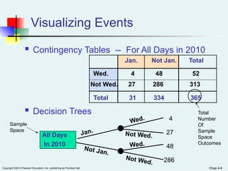
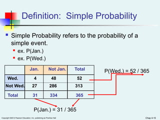
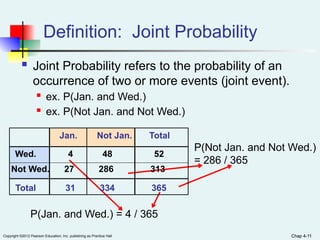
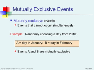
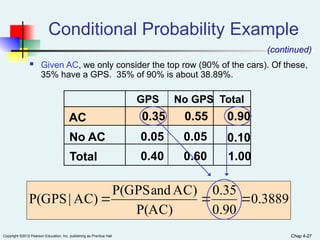
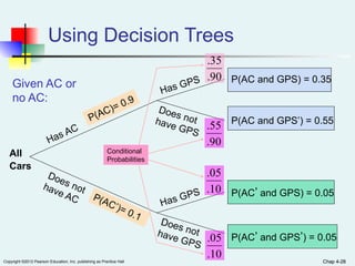
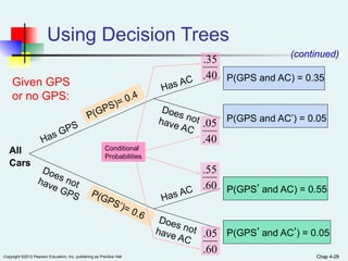
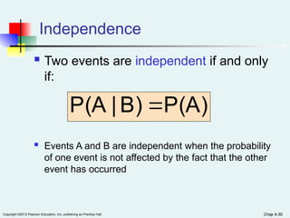
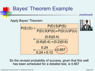
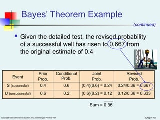
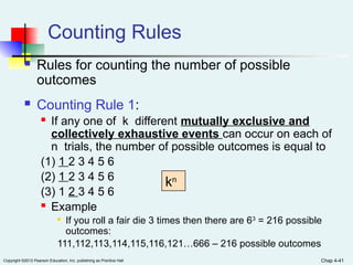
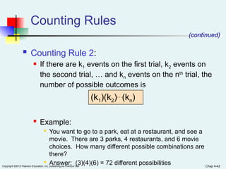
Basic Business Statistics 12-th edition,Chapter 4,Basic Probability

Copyright ©2012 Pearson Education, Inc. publishing as Prentice Hall Chap 4-1
Chap 4-1
Chapter 4
Basic Probability
Basic Business Statistics
12th
Edition

Chap 4-2
Learning Objectives
In this chapter, you learn:
 Basic probability concepts
 Conditional probability
 To use Bayes’ Theorem to revise probabilities
 Various counting rules

Chap 4-3
Basic Probability Concepts
 Probability – the chance that an uncertain event
will occur (always between 0 and 1)
 Impossible Event – an event that has no
chance of occurring (probability = 0)
 Certain Event – an event that is sure to occur
(probability = 1)

Chap 4-4
Assessing Probability
There are three approaches to assessing the
probability of an uncertain event:
1. a priori -- based on prior knowledge of the process
2. empirical probability -- based on observed data
3. subjective probability
outcomes
elementary
of
number
total
occur
can
event
the
ways
of
number
T
X


based on a combination of an individual’s past experience,
personal opinion, and analysis of a particular situation
outcomes
elementary
of
number
total
occur
can
event
the
ways
of
number

Assuming
all
outcomes
are equally
likely
probability of occurrence
probability of occurrence

Chap 4-5
Example of a priori probability
When randomly selecting a day from the year 2010
what is the probability the day is in January?
2010
in
days
of
number
total
January
in
days
of
number
January
In
Day
of
y
Probabilit 

T
X
365
31
2010
in
days
365
January
in
days
31


T
X

Chap 4-6
Example of empirical probability
Taking Stats Not Taking
Stats
Total
Male 84 145 229
Female 76 134 210
Total 160 279 439
Find the probability of selecting a male taking statistics
from the population described in the following table:
191
.
0
439
84
people
of
number
total
stats
taking
males
of
number



Probability of male taking stats

Chap 4-7
Events
Each possible outcome of a variable is an event.
 Simple event
 An event described by a single characteristic
 e.g., A day in January from all days in 2010
 Joint event
 An event described by two or more characteristics
 e.g. A day in January that is also a Wednesday from all days in 2010
 Complement of an event A (denoted A’)
 All events that are not part of event A
 e.g., All days from 2010 that are not in January

Chap 4-8
Sample Space
The Sample Space is the collection of all
possible events of a random experiment.
e.g. All 6 faces of a die:
e.g. All 52 cards of a bridge deck:

Chap 4-9
Visualizing Events
 Contingency Tables -- For All Days in 2010
 Decision Trees
All Days
In 2010
Not Jan.
Jan.
Not Wed.
Wed.
Wed.
Not Wed.
Sample
Space
Total
Number
Of
Sample
Space
Outcomes
Not Wed. 27 286 313
Wed. 4 48 52
Total 31 334 365
Jan. Not Jan. Total
4
27
48
286

Chap 4-10
Definition: Simple Probability
 Simple Probability refers to the probability of a
simple event.
 ex. P(Jan.)
 ex. P(Wed.)
P(Jan.) = 31 / 365
P(Wed.) = 52 / 365
Not Wed. 27 286 313
Wed. 4 48 52
Total 31 334 365
Jan. Not Jan. Total

Chap 4-11
Definition: Joint Probability
 Joint Probability refers to the probability of an
occurrence of two or more events (joint event).
 ex. P(Jan. and Wed.)
 ex. P(Not Jan. and Not Wed.)
P(Jan. and Wed.) = 4 / 365
P(Not Jan. and Not Wed.)
= 286 / 365
Not Wed. 27 286 313
Wed. 4 48 52
Total 31 334 365
Jan. Not Jan. Total

Chap 4-12
Mutually Exclusive Events
 Mutually exclusive events
 Events that cannot occur simultaneously
Example: Randomly choosing a day from 2010
A = day in January; B = day in February
 Events A and B are mutually exclusive

Chap 4-13
Collectively Exhaustive Events
 Collectively exhaustive events
 One of the events must occur

The set of events covers the entire sample space
Example: Randomly choose a day from 2010
A = Weekday; B = Weekend;
C = January; D = Spring;
 Events A, B, C and D are collectively exhaustive
(but not mutually exclusive – a weekday can be in
January or in Spring)
 Events A and B are collectively exhaustive and
also mutually exclusive

Chap 4-14
Computing Joint and
Marginal Probabilities
 The probability of a joint event, A and B:
 Computing a marginal (or simple) probability:

Where B1, B2, …, Bk are k mutually exclusive and collectively
exhaustive events
outcomes
elementary
of
number
total
B
and
A
satisfying
outcomes
of
number
)
B
and
A
(
P 
)
B
d
an
P(A
)
B
and
P(A
)
B
and
P(A
P(A) k
2
1 


 

Chap 4-15
Joint Probability Example
P(Jan. and Wed.)
365
4
2010
in
days
of
number
total
Wed.
are
and
Jan.
in
are
that
days
of
number


Not Wed. 27 286 313
Wed. 4 48 52
Total 31 334 365
Jan. Not Jan. Total

Chap 4-16
Marginal Probability Example
P(Wed.)
365
52
365
48
365
4
)
Wed.
and
Jan.
P(Not
Wed.)
and
Jan.
( 



P
Not Wed. 27 286 313
Wed. 4 48 52
Total 31 334 365
Jan. Not Jan. Total

Chap 4-17
P(A1 and B2) P(A1)
Total
Event
Marginal & Joint Probabilities In A
Contingency Table
P(A2 and B1)
P(A1 and B1)
Event
Total 1
Joint Probabilities Marginal (Simple) Probabilities
A1
A2
B1 B2
P(B1) P(B2)
P(A2 and B2) P(A2)

Chap 4-18
Probability Summary So Far
 Probability is the numerical measure
of the likelihood that an event will
occur
 The probability of any event must
be between 0 and 1, inclusively
 The sum of the probabilities of all
mutually exclusive and collectively
exhaustive events is 1
Certain
Impossible
0.5
1
0
0 ≤ P(A) ≤ 1 For any event A
1
P(C)
P(B)
P(A) 


If A, B, and C are mutually exclusive and
collectively exhaustive

Chap 4-19
General Addition Rule
P(A or B) = P(A) + P(B) - P(A and B)
General Addition Rule:
If A and B are mutually exclusive, then
P(A and B) = 0, so the rule can be simplified:
P(A or B) = P(A) + P(B)
For mutually exclusive events A and B

Chap 4-22
General Addition Rule Example
P(Jan. or Wed.) = P(Jan.) + P(Wed.) - P(Jan. and Wed.)
= 31/365 + 52/365 - 4/365 = 79/365
Don’t count
the four
Wednesdays
in January
twice!
Not Wed. 27 286 313
Wed. 4 48 52
Total 31 334 365
Jan. Not Jan. Total

Chap 4-23
Computing Conditional
Probabilities
 A conditional probability is the probability of one
event, given that another event has occurred:
P(B)
B)
and
P(A
B)
|
P(A 
P(A)
B)
and
P(A
A)
|
P(B 
Where P(A and B) = joint probability of A and B
P(A) = marginal or simple probability of A
P(B) = marginal or simple probability of B
The conditional
probability of A given
that B has occurred
The conditional
probability of B given
that A has occurred

Chap 4-25
 What is the probability that a car has a GPS
given that it has AC ?
i.e., we want to find P(GPS | AC)
Conditional Probability Example
 Of the cars on a used car lot, 90% have air
conditioning (AC) and 40% have a GPS. 35% of
the cars have both.

Chap 4-26
 Of the cars on a used car lot, 90% have air conditioning
(AC) and 40% have a GPS.
35% of the cars have both.
No GPS
GPS Total
AC 0.35 0.55 0.90
No AC 0.05 0.05 0.10
Total 0.40 0.60 1.00
0.3889
0.90
0.35
P(AC)
AC)
and
P(GPS
AC)
|
P(GPS 


(continued)

Chap 4-27
 Given AC, we only consider the top row (90% of the cars). Of these,
35% have a GPS. 35% of 90% is about 38.89%.
(continued)
No GPS
GPS Total
AC 0.35 0.55 0.90
No AC 0.05 0.05 0.10
Total 0.40 0.60 1.00
0.3889
0.90
0.35
P(AC)
AC)
and
P(GPS
AC)
|
P(GPS 



Chap 4-28
Using Decision Trees
Has AC
Does not
have AC
Has GPS
Does not
have GPS
Has GPS
Does not
have GPS
P(AC)= 0.9
P(AC’)= 0.1
P(AC and GPS) = 0.35
P(AC and GPS’) = 0.55
P(AC’ and GPS’) = 0.05
P(AC’ and GPS) = 0.05
90
.
55
.
10
.
05
.
10
.
05
.
All
Cars
90
.
35
.
Given AC or
no AC:
Conditional
Probabilities

Chap 4-29
Using Decision Trees
Has GPS
Does not
have GPS
Has AC
Does not
have AC
Has AC
Does not
have AC
P(GPS)= 0.4
P(GPS’)= 0.6
P(GPS and AC) = 0.35
P(GPS and AC’) = 0.05
P(GPS’ and AC’) = 0.05
P(GPS’ and AC) = 0.55
40
.
05
.
60
.
55
.
60
.
05
.
All
Cars
40
.
35
.
Given GPS
or no GPS:
(continued)
Conditional
Probabilities

Chap 4-30
Independence
 Two events are independent if and only
if:
 Events A and B are independent when the probability
of one event is not affected by the fact that the other
event has occurred
P(A)
B)
|
P(A 

Copyright ©2012 Pearson Education, Inc. publishing as Prentice Hall
The difference between mutually
exclusive and independent events
 a mutually exclusive event can simply be defined as a
situation when two events cannot occur at same time whereas
independent event occurs when one event remains unaffected by
the occurrence of the other event. Suppose an event does not
take place that does not stop other events from happening. It
is important to note here that mutually exclusive events cannot be
independent unless the probability of one of the events is zero.
 The mathematical formula for mutually exclusive events can be
represented as P(X and Y) = 0
 The mathematical formula for independent events can be defined
as P(X and Y) = P(X) P(Y)
 Example: when a coin is a tossed and there are two events that
can occur, either it will be a head or a tail. Hence, both the events
here are mutually exclusive. But if we take two separate coins and
flip them, then the occurrence of Head or Tail on both the coins are
independent to each other.
Chap 4-31

Chap 4-32
Multiplication Rules
 Multiplication rule for two events A and B:
P(B)
B)
|
P(A
B)
and
P(A 
P(A)
B)
|
P(A 
Note: If A and B are independent, then
and the multiplication rule simplifies to
P(B)
P(A)
B)
and
P(A 

Chap 4-33
Marginal Probability
 Marginal probability for event A:

Where B1, B2, …, Bk are k mutually exclusive and
collectively exhaustive events
)
P(B
)
B
|
P(A
)
P(B
)
B
|
P(A
)
P(B
)
B
|
P(A
P(A) k
k
2
2
1
1 


 

Chap 4-34
Bayes’ Theorem
 Bayes’ Theorem is used to revise previously
calculated probabilities based on new
information.
 Developed by Thomas Bayes in the 18th
Century.
 It is an extension of conditional probability.

Chap 4-36
Bayes’ Theorem Example
 A drilling company has estimated a 40%
chance of striking oil for their new well.
 A detailed test has been scheduled for more
information. Historically, 60% of successful
wells have had detailed tests, and 20% of
unsuccessful wells have had detailed tests.
 Given that this well has been scheduled for a
detailed test, what is the probability
that the well will be successful?

Chap 4-37
 Let S = successful well
U = unsuccessful well
 P(S) =0.4, P(U) =0.6 (prior probabilities)
 Define the detailed test event as D
 Conditional probabilities:
P(D|S) = 0.6 P(D|U) =0.2
 Goal is to find P(S|D)=?
(continued)

Chap 4-38
 Let S = successful well
U = unsuccessful well
 P(S) = 0.4 , P(U) = 0.6 (prior probabilities)
 Define the detailed test event as D
 Conditional probabilities:
P(D|S) = 0.6 P(D|U) = 0.2
 Goal is to find P(S|D)
(continued)

Chap 4-39
0.667
0.12
0.24
0.24
(0.2)(0.6)
(0.6)(0.4)
(0.6)(0.4)
U)P(U)
|
P(D
S)P(S)
|
P(D
S)P(S)
|
P(D
D)
|
P(S







(continued)
Apply Bayes’ Theorem:
So the revised probability of success, given that this well
has been scheduled for a detailed test, is 0.667

Chap 4-40
 Given the detailed test, the revised probability
of a successful well has risen to 0.667 from
the original estimate of 0.4
Event
Prior
Prob.
Conditional
Prob.
Joint
Prob.
Revised
Prob.
S (successful) 0.4 0.6 (0.4)(0.6) = 0.24 0.24/0.36 = 0.667
U (unsuccessful) 0.6 0.2 (0.6)(0.2) = 0.12 0.12/0.36 = 0.333
Sum = 0.36
(continued)

Chap 4-41
Counting Rules
 Rules for counting the number of possible
outcomes
 Counting Rule 1:
 If any one of k different mutually exclusive and
collectively exhaustive events can occur on each of
n trials, the number of possible outcomes is equal to
(1) 1 2 3 4 5 6
(2) 1 2 3 4 5 6
(3) 1 2 3 4 5 6
 Example

If you roll a fair die 3 times then there are 63
= 216 possible
outcomes:
111,112,113,114,115,116,121…666 – 216 possible outcomes
kn

Chap 4-42
Counting Rules
 If there are k1 events on the first trial, k2 events on
the second trial, … and kn events on the nth
trial, the
number of possible outcomes is
 Example:

You want to go to a park, eat at a restaurant, and see a
movie. There are 3 parks, 4 restaurants, and 6 movie
choices. How many different possible combinations are
there?

Answer: (3)(4)(6) = 72 different possibilities
(k1)(k2)…
(kn)
(continued)

Chap 4-43
Counting Rules
 The number of ways that n items can be arranged in
order is
 Example:

You have five books to put on a bookshelf. How many
different ways can these books be placed on the shelf?

Answer: 5! = (5)(4)(3)(2)(1) = 120 different possibilities
n! = (n)(n – 1)…
(1)
(continued)

A B C D
E
Chap 4-44
 ABCDE ….. 120 possible outcomes
 ACBDE
 ADBCE
 AEBCD
 BACDE

Chap 4-45
Counting Rules
 Permutations: The number of ways of arranging X
objects selected from n objects in order is
 Example:

You have five books and are going to put three on a
bookshelf. How many different ways can the books be
ordered on the bookshelf?

Answer: different
possibilities
(continued)
X)!
(n
n!
Px
n


60
2
120
3)!
(5
5!
X)!
(n
n!
Px
n 






A B C D
E
Chap 4-46
 ABC
 ACB
 BAC
 BCA
 CAB
 CBA
 ABD
 ADB
 BAD
 BDA
 DAB
 DBA
 ABE
 AEB
 BAE
 BEA
 EAB
 EBA
 …

Chap 4-47
Counting Rules
 Combinations: The number of ways of selecting X
objects from n objects, irrespective of order, is
 Example:

You have five books and are going to randomly select three
to read. How many different combinations of books might
you select?

Answer: different
possibilities
(continued)
X)!
(n
X!
n!
Cx
n


10
(6)(2)
120
3)!
(5
3!
5!
X)!
(n
X!
n!
Cx
n 






A B C D
E
Chap 4-48
1st
combination:
 ABC
 ACB
 BAC
 BCA
 CAB
 CBA
2nd
combination:
 ABD
 ADB
 BAD
 BDA
 DAB
 DBA
3rd
combination:
 ABE
 AEB
 BAE
 BEA
 EAB
 EBA
 …

Chap 4-49
Chapter Summary
 Discussed basic probability concepts
 Sample spaces and events, contingency tables, simple
probability, and joint probability
 Examined basic probability rules
 General addition rule, addition rule for mutually exclusive events,
rule for collectively exhaustive events
 Defined conditional probability
 Statistical independence, marginal probability, decision trees,
and the multiplication rule
 Discussed Bayes’ theorem
 Discussed various counting rules

Basic Business Statistics 12-th edition,Chapter 4,Basic Probability

More Related Content

What's hot

Similar to Basic Business Statistics 12-th edition,Chapter 4,Basic Probability

Recently uploaded

Basic Business Statistics 12-th edition,Chapter 4,Basic Probability

Editor's Notes