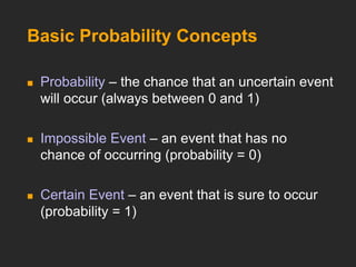
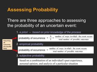
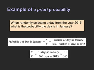
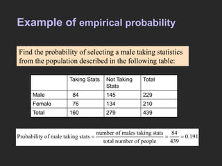
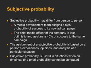
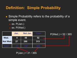
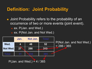
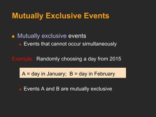
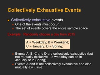
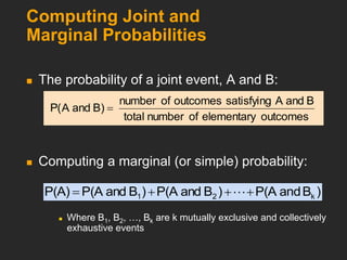
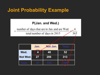
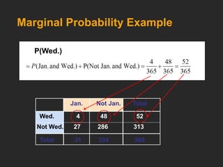
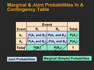
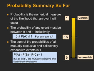
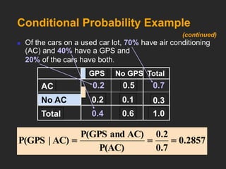
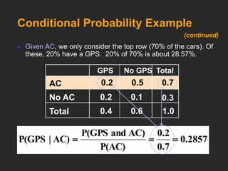
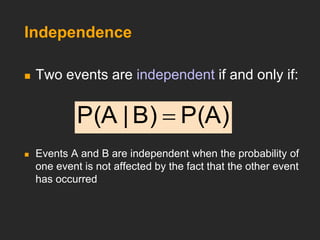
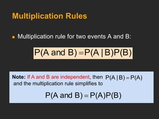
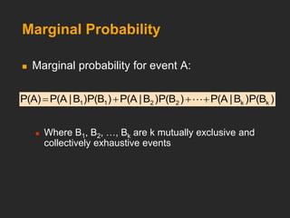
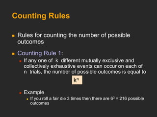
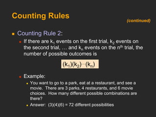
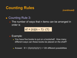
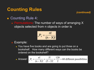
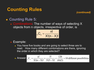
JAMES FRANCIS A. GOSE,
MBA
BASIC
CONCEPT OF
PROBABILITY
Objectives
The objectives for this chapter are:
 To understand basic probability concepts.
 To understand conditional probability
 To be able to use Bayes’ Theorem to revise
probabilities
 To learn various counting rules
Basic Probability Concepts
 Probability – the chance that an uncertain event
will occur (always between 0 and 1)
 Impossible Event – an event that has no
chance of occurring (probability = 0)
 Certain Event – an event that is sure to occur
(probability = 1)
probability of occurrence
Assessing Probability
There are three approaches to assessing
the probability of an uncertain event:
1. a priori -- based on prior knowledge of the process
2. empirical probability
3. subjective probability
outcomes
possible
of
number
total
occurs
event
the
in which
ways
of
number
T
X


based on a combination of an individual’s past experience,
personal opinion, and analysis of a particular situation
outcomes
possible
of
number
total
occurs
event
the
in which
ways
of
number

Assuming
all
outcomes
are equally
likely
probability of occurrence
Example of a priori probability
365
31
2015
in
days
365
January
in
days
31


T
X
When randomly selecting a day from the year 2015
what is the probability the day is in January?
2015
in
days
of
number
total
January
in
days
of
number
January
In
Day
of
y
Probabilit 

T
X
Example of empirical probability
number of males taking stats 84
0.191
total num
Proba
ber o
bility of mal
f peopl
e taking
e 439
stats   
Taking Stats Not Taking
Stats
Total
Male 84 145 229
Female 76 134 210
Total 160 279 439
Find the probability of selecting a male taking statistics
from the population described in the following table:
Subjective probability
 Subjective probability may differ from person to person
 A media development team assigns a 60%
probability of success to its new ad campaign.
 The chief media officer of the company is less
optimistic and assigns a 40% of success to the same
campaign
 The assignment of a subjective probability is based on a
person’s experiences, opinions, and analysis of a
particular situation
 Subjective probability is useful in situations when an
empirical or a priori probability cannot be computed
Events
Each possible outcome of a variable is an event.
 Simple event
 An event described by a single characteristic
 e.g., A day in January from all days in 2015
 Joint event
 An event described by two or more characteristics
 e.g. A day in January that is also a Wednesday from all days in
2015
 Complement of an event A (denoted A’)
 All events that are not part of event A
 e.g., All days from 2015 that are not in January
The Sample Space is the collection of all
possible events
e.g. All 6 faces of a die:
e.g. All 52 cards of a bridge deck:
Sample Space
Organizing & Visualizing Events
 Venn Diagram For All Days In 2015
Sample Space (All Days
In 2015)
January Days
Wednesdays
Days That Are In January and Are
Wednesdays
Organizing & Visualizing Events
 Contingency Tables -- For All Days in 2015
 Decision Trees
All Days
In 2015
Sample
Space
Total
Number
Of
Sample
Space
Outcomes
4
27
48
286
(continued)
Definition: Simple Probability
 Simple Probability refers to the probability of a
simple event.
 ex. P(Jan.)
 ex. P(Wed.)
P(Jan.) = 31 / 365
P(Wed.) = 52 / 365
Not Wed. 27 286 313
Wed. 4 48 52
Total 31 334 365
Jan. Not Jan. Total
Definition: Joint Probability
 Joint Probability refers to the probability of an
occurrence of two or more events (joint event).
 ex. P(Jan. and Wed.)
 ex. P(Not Jan. and Not Wed.)
P(Jan. and Wed.) = 4 / 365
P(Not Jan. and Not Wed.)
= 286 / 365
Not Wed. 27 286 313
Wed. 4 48 52
Total 31 334 365
Jan. Not Jan. Total
Mutually Exclusive Events
 Mutually exclusive events
 Events that cannot occur simultaneously
Example: Randomly choosing a day from 2015
A = day in January; B = day in February
 Events A and B are mutually exclusive
Collectively Exhaustive Events
 Collectively exhaustive events
 One of the events must occur
 The set of events covers the entire sample space
Example: Randomly choose a day from 2015
A = Weekday; B = Weekend;
C = January; D = Spring;
 Events A, B, C and D are collectively exhaustive (but
not mutually exclusive – a weekday can be in
January or in Spring)
 Events A and B are collectively exhaustive and also
mutually exclusive
Computing Joint and
Marginal Probabilities
 The probability of a joint event, A and B:
 Computing a marginal (or simple) probability:
 Where B1, B2, …, Bk are k mutually exclusive and collectively
exhaustive events
outcomes
elementary
of
number
total
B
and
A
satisfying
outcomes
of
number
)
B
and
A
(
P 
)
B
d
an
P(A
)
B
and
P(A
)
B
and
P(A
P(A) k
2
1 


 
Joint Probability Example
Not Wed. 27 286 313
Wed. 4 48 52
Total 31 334 365
Jan. Not Jan. Total
Not Wed. 27 286 313
Wed. 4 48 52
Total 31 334 365
Jan. Not Jan. Total
Marginal Probability Example
P(A1 and B2) P(A1)
Total
Event
Marginal & Joint Probabilities In A
Contingency Table
P(A2 and B1)
P(A1 and B1)
Event
Total 1
Joint Probabilities Marginal (Simple) Probabilities
A1
A2
B1 B2
P(B1) P(B2)
P(A2 and B2) P(A2)
Probability Summary So Far
 Probability is the numerical measure
of the likelihood that an event will
occur
 The probability of any event must be
between 0 and 1, inclusively
 The sum of the probabilities of all
mutually exclusive and collectively
exhaustive events is 1
Certain
Impossible
0.5
1
0
0 ≤ P(A) ≤ 1 For any event A
1
P(C)
P(B)
P(A) 


If A, B, and C are mutually exclusive and
collectively exhaustive
General Addition Rule
P(A or B) = P(A) + P(B) - P(A and B)
General Addition Rule:
If A and B are mutually exclusive, then
P(A and B) = 0, so the rule can be simplified:
P(A or B) = P(A) + P(B)
For mutually exclusive events A and B
General Addition Rule Example
P(Jan. or Wed.) = P(Jan.) + P(Wed.) - P(Jan. and Wed.)
= 31/365 + 52/365 - 4/365 = 79/365
Don’t count
the four
Wednesdays
in January
twice!
Not Wed. 27 286 313
Wed. 4 48 52
Total 31 334 365
Jan. Not Jan. Total
Computing Conditional
Probabilities
 A conditional probability is the probability of one
event, given that another event has occurred:
P(B)
B)
and
P(A
B)
|
P(A 
P(A)
B)
and
P(A
A)
|
P(B 
Where P(A and B) = joint probability of A and B
P(A) = marginal or simple probability of A
P(B) = marginal or simple probability of B
The conditional
probability of A given
that B has occurred
The conditional
probability of B given
that A has occurred
Conditional Probability Example
 What is the probability that a car has a GPS,
given that it has AC ?
i.e., we want to find P(GPS | AC)
 Of the cars on a used car lot, 70% have air
conditioning (AC) and 40% have a GPS. 20%
of the cars have both.
Conditional Probability Example
No GPS
GPS Total
AC 0.2 0.5 0.7
No AC 0.2 0.1 0.3
Total 0.4 0.6 1.0
 Of the cars on a used car lot, 70% have air conditioning
(AC) and 40% have a GPS and
20% of the cars have both.
0.2857
0.7
0.2
P(AC)
AC)
and
P(GPS
AC)
|
P(GPS 


(continued)
Conditional Probability Example
No GPS
GPS Total
AC 0.2 0.5 0.7
No AC 0.2 0.1 0.3
Total 0.4 0.6 1.0
 Given AC, we only consider the top row (70% of the cars). Of
these, 20% have a GPS. 20% of 70% is about 28.57%.
0.2857
0.7
0.2
P(AC)
AC)
and
P(GPS
AC)
|
P(GPS 


(continued)
Independence
 Two events are independent if and only if:
 Events A and B are independent when the probability of
one event is not affected by the fact that the other event
has occurred
P(A)
B)
|
P(A 
Multiplication Rules
 Multiplication rule for two events A and B:
P(B)
B)
|
P(A
B)
and
P(A 
P(A)
B)
|
P(A 
Note: If A and B are independent, then
and the multiplication rule simplifies to
P(B)
P(A)
B)
and
P(A 
Marginal Probability
 Marginal probability for event A:
 Where B1, B2, …, Bk are k mutually exclusive and
collectively exhaustive events
)
P(B
)
B
|
P(A
)
P(B
)
B
|
P(A
)
P(B
)
B
|
P(A
P(A) k
k
2
2
1
1 


 
Counting Rules Are Often Useful In
Computing Probabilities
 In many cases, there are a large number of
possible outcomes.
 Counting rules can be used in these cases to
help compute probabilities.
Counting Rules
 Rules for counting the number of possible
outcomes
 Counting Rule 1:
 If any one of k different mutually exclusive and
collectively exhaustive events can occur on each of
n trials, the number of possible outcomes is equal to
 Example
 If you roll a fair die 3 times then there are 63 = 216 possible
outcomes
kn
Counting Rules
 Counting Rule 2:
 If there are k1 events on the first trial, k2 events on
the second trial, … and kn events on the nth trial, the
number of possible outcomes is
 Example:
 You want to go to a park, eat at a restaurant, and see a
movie. There are 3 parks, 4 restaurants, and 6 movie
choices. How many different possible combinations are
there?
 Answer: (3)(4)(6) = 72 different possibilities
(k1)(k2)…(kn)
(continued)
Counting Rules
 Counting Rule 3:
 The number of ways that n items can be arranged in
order is
 Example:
 You have five books to put on a bookshelf. How many
different ways can these books be placed on the shelf?
 Answer: 5! = (5)(4)(3)(2)(1) = 120 different possibilities
n! = (n)(n – 1)…(1)
(continued)
Counting Rules
 Counting Rule 4:
 Permutations: The number of ways of arranging X
objects selected from n objects in order is
 Example:
 You have five books and are going to put three on a
bookshelf. How many different ways can the books be
ordered on the bookshelf?
 Answer:
X)!
(n
n!
Px
n


n x
n! 5! 120
P 60
(n X)! (5 3)! 2
different possibilities
   
 
(continued)
Counting Rules
 Counting Rule 5:
 Combinations: The number of ways of selecting X
objects from n objects, irrespective of order, is
 Example:
 You have five books and are going to select three are to
read. How many different combinations are there, ignoring
the order in which they are selected?
 Answer:
X)!
(n
X!
n!
Cx
n


n x
n! 5! 120
C 10
X!(n X)! 3!(5 3)! (6)
different possi
(
b
2)
ilities
   
 
(continued)
Chapter Summary
In this chapter we covered:
 Understanding basic probability concepts.
 Understanding conditional probability
 Using Bayes’ Theorem to revise probabilities
 Various counting rules

BASIC CONCEPT OF PROBABILITY by Elem Stppt

  • 1.
    JAMES FRANCIS A.GOSE, MBA BASIC CONCEPT OF PROBABILITY
  • 2.
    Objectives The objectives forthis chapter are:  To understand basic probability concepts.  To understand conditional probability  To be able to use Bayes’ Theorem to revise probabilities  To learn various counting rules
  • 3.
    Basic Probability Concepts Probability – the chance that an uncertain event will occur (always between 0 and 1)  Impossible Event – an event that has no chance of occurring (probability = 0)  Certain Event – an event that is sure to occur (probability = 1)
  • 4.
    probability of occurrence AssessingProbability There are three approaches to assessing the probability of an uncertain event: 1. a priori -- based on prior knowledge of the process 2. empirical probability 3. subjective probability outcomes possible of number total occurs event the in which ways of number T X   based on a combination of an individual’s past experience, personal opinion, and analysis of a particular situation outcomes possible of number total occurs event the in which ways of number  Assuming all outcomes are equally likely probability of occurrence
  • 5.
    Example of apriori probability 365 31 2015 in days 365 January in days 31   T X When randomly selecting a day from the year 2015 what is the probability the day is in January? 2015 in days of number total January in days of number January In Day of y Probabilit   T X
  • 6.
    Example of empiricalprobability number of males taking stats 84 0.191 total num Proba ber o bility of mal f peopl e taking e 439 stats    Taking Stats Not Taking Stats Total Male 84 145 229 Female 76 134 210 Total 160 279 439 Find the probability of selecting a male taking statistics from the population described in the following table:
  • 7.
    Subjective probability  Subjectiveprobability may differ from person to person  A media development team assigns a 60% probability of success to its new ad campaign.  The chief media officer of the company is less optimistic and assigns a 40% of success to the same campaign  The assignment of a subjective probability is based on a person’s experiences, opinions, and analysis of a particular situation  Subjective probability is useful in situations when an empirical or a priori probability cannot be computed
  • 8.
    Events Each possible outcomeof a variable is an event.  Simple event  An event described by a single characteristic  e.g., A day in January from all days in 2015  Joint event  An event described by two or more characteristics  e.g. A day in January that is also a Wednesday from all days in 2015  Complement of an event A (denoted A’)  All events that are not part of event A  e.g., All days from 2015 that are not in January
  • 9.
    The Sample Spaceis the collection of all possible events e.g. All 6 faces of a die: e.g. All 52 cards of a bridge deck: Sample Space
  • 10.
    Organizing & VisualizingEvents  Venn Diagram For All Days In 2015 Sample Space (All Days In 2015) January Days Wednesdays Days That Are In January and Are Wednesdays
  • 11.
    Organizing & VisualizingEvents  Contingency Tables -- For All Days in 2015  Decision Trees All Days In 2015 Sample Space Total Number Of Sample Space Outcomes 4 27 48 286 (continued)
  • 12.
    Definition: Simple Probability Simple Probability refers to the probability of a simple event.  ex. P(Jan.)  ex. P(Wed.) P(Jan.) = 31 / 365 P(Wed.) = 52 / 365 Not Wed. 27 286 313 Wed. 4 48 52 Total 31 334 365 Jan. Not Jan. Total
  • 13.
    Definition: Joint Probability Joint Probability refers to the probability of an occurrence of two or more events (joint event).  ex. P(Jan. and Wed.)  ex. P(Not Jan. and Not Wed.) P(Jan. and Wed.) = 4 / 365 P(Not Jan. and Not Wed.) = 286 / 365 Not Wed. 27 286 313 Wed. 4 48 52 Total 31 334 365 Jan. Not Jan. Total
  • 14.
    Mutually Exclusive Events Mutually exclusive events  Events that cannot occur simultaneously Example: Randomly choosing a day from 2015 A = day in January; B = day in February  Events A and B are mutually exclusive
  • 15.
    Collectively Exhaustive Events Collectively exhaustive events  One of the events must occur  The set of events covers the entire sample space Example: Randomly choose a day from 2015 A = Weekday; B = Weekend; C = January; D = Spring;  Events A, B, C and D are collectively exhaustive (but not mutually exclusive – a weekday can be in January or in Spring)  Events A and B are collectively exhaustive and also mutually exclusive
  • 16.
    Computing Joint and MarginalProbabilities  The probability of a joint event, A and B:  Computing a marginal (or simple) probability:  Where B1, B2, …, Bk are k mutually exclusive and collectively exhaustive events outcomes elementary of number total B and A satisfying outcomes of number ) B and A ( P  ) B d an P(A ) B and P(A ) B and P(A P(A) k 2 1     
  • 17.
    Joint Probability Example NotWed. 27 286 313 Wed. 4 48 52 Total 31 334 365 Jan. Not Jan. Total
  • 18.
    Not Wed. 27286 313 Wed. 4 48 52 Total 31 334 365 Jan. Not Jan. Total Marginal Probability Example
  • 19.
    P(A1 and B2)P(A1) Total Event Marginal & Joint Probabilities In A Contingency Table P(A2 and B1) P(A1 and B1) Event Total 1 Joint Probabilities Marginal (Simple) Probabilities A1 A2 B1 B2 P(B1) P(B2) P(A2 and B2) P(A2)
  • 20.
    Probability Summary SoFar  Probability is the numerical measure of the likelihood that an event will occur  The probability of any event must be between 0 and 1, inclusively  The sum of the probabilities of all mutually exclusive and collectively exhaustive events is 1 Certain Impossible 0.5 1 0 0 ≤ P(A) ≤ 1 For any event A 1 P(C) P(B) P(A)    If A, B, and C are mutually exclusive and collectively exhaustive
  • 21.
    General Addition Rule P(Aor B) = P(A) + P(B) - P(A and B) General Addition Rule: If A and B are mutually exclusive, then P(A and B) = 0, so the rule can be simplified: P(A or B) = P(A) + P(B) For mutually exclusive events A and B
  • 22.
    General Addition RuleExample P(Jan. or Wed.) = P(Jan.) + P(Wed.) - P(Jan. and Wed.) = 31/365 + 52/365 - 4/365 = 79/365 Don’t count the four Wednesdays in January twice! Not Wed. 27 286 313 Wed. 4 48 52 Total 31 334 365 Jan. Not Jan. Total
  • 23.
    Computing Conditional Probabilities  Aconditional probability is the probability of one event, given that another event has occurred: P(B) B) and P(A B) | P(A  P(A) B) and P(A A) | P(B  Where P(A and B) = joint probability of A and B P(A) = marginal or simple probability of A P(B) = marginal or simple probability of B The conditional probability of A given that B has occurred The conditional probability of B given that A has occurred
  • 24.
    Conditional Probability Example What is the probability that a car has a GPS, given that it has AC ? i.e., we want to find P(GPS | AC)  Of the cars on a used car lot, 70% have air conditioning (AC) and 40% have a GPS. 20% of the cars have both.
  • 25.
    Conditional Probability Example NoGPS GPS Total AC 0.2 0.5 0.7 No AC 0.2 0.1 0.3 Total 0.4 0.6 1.0  Of the cars on a used car lot, 70% have air conditioning (AC) and 40% have a GPS and 20% of the cars have both. 0.2857 0.7 0.2 P(AC) AC) and P(GPS AC) | P(GPS    (continued)
  • 26.
    Conditional Probability Example NoGPS GPS Total AC 0.2 0.5 0.7 No AC 0.2 0.1 0.3 Total 0.4 0.6 1.0  Given AC, we only consider the top row (70% of the cars). Of these, 20% have a GPS. 20% of 70% is about 28.57%. 0.2857 0.7 0.2 P(AC) AC) and P(GPS AC) | P(GPS    (continued)
  • 27.
    Independence  Two eventsare independent if and only if:  Events A and B are independent when the probability of one event is not affected by the fact that the other event has occurred P(A) B) | P(A 
  • 28.
    Multiplication Rules  Multiplicationrule for two events A and B: P(B) B) | P(A B) and P(A  P(A) B) | P(A  Note: If A and B are independent, then and the multiplication rule simplifies to P(B) P(A) B) and P(A 
  • 29.
    Marginal Probability  Marginalprobability for event A:  Where B1, B2, …, Bk are k mutually exclusive and collectively exhaustive events ) P(B ) B | P(A ) P(B ) B | P(A ) P(B ) B | P(A P(A) k k 2 2 1 1     
  • 30.
    Counting Rules AreOften Useful In Computing Probabilities  In many cases, there are a large number of possible outcomes.  Counting rules can be used in these cases to help compute probabilities.
  • 31.
    Counting Rules  Rulesfor counting the number of possible outcomes  Counting Rule 1:  If any one of k different mutually exclusive and collectively exhaustive events can occur on each of n trials, the number of possible outcomes is equal to  Example  If you roll a fair die 3 times then there are 63 = 216 possible outcomes kn
  • 32.
    Counting Rules  CountingRule 2:  If there are k1 events on the first trial, k2 events on the second trial, … and kn events on the nth trial, the number of possible outcomes is  Example:  You want to go to a park, eat at a restaurant, and see a movie. There are 3 parks, 4 restaurants, and 6 movie choices. How many different possible combinations are there?  Answer: (3)(4)(6) = 72 different possibilities (k1)(k2)…(kn) (continued)
  • 33.
    Counting Rules  CountingRule 3:  The number of ways that n items can be arranged in order is  Example:  You have five books to put on a bookshelf. How many different ways can these books be placed on the shelf?  Answer: 5! = (5)(4)(3)(2)(1) = 120 different possibilities n! = (n)(n – 1)…(1) (continued)
  • 34.
    Counting Rules  CountingRule 4:  Permutations: The number of ways of arranging X objects selected from n objects in order is  Example:  You have five books and are going to put three on a bookshelf. How many different ways can the books be ordered on the bookshelf?  Answer: X)! (n n! Px n   n x n! 5! 120 P 60 (n X)! (5 3)! 2 different possibilities       (continued)
  • 35.
    Counting Rules  CountingRule 5:  Combinations: The number of ways of selecting X objects from n objects, irrespective of order, is  Example:  You have five books and are going to select three are to read. How many different combinations are there, ignoring the order in which they are selected?  Answer: X)! (n X! n! Cx n   n x n! 5! 120 C 10 X!(n X)! 3!(5 3)! (6) different possi ( b 2) ilities       (continued)
  • 36.
    Chapter Summary In thischapter we covered:  Understanding basic probability concepts.  Understanding conditional probability  Using Bayes’ Theorem to revise probabilities  Various counting rules