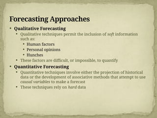
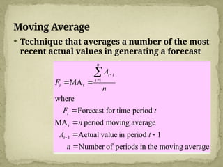
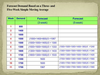
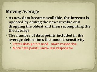
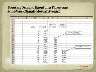
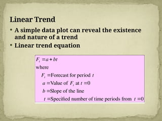
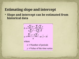
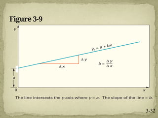
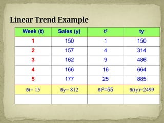
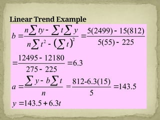
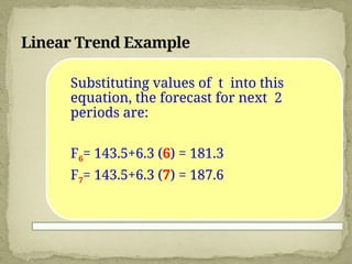
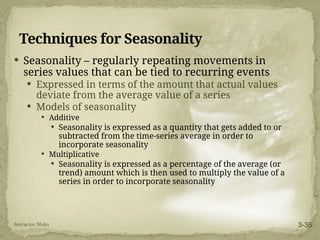
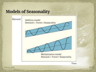
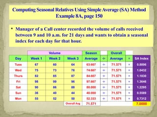
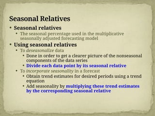
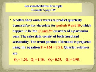
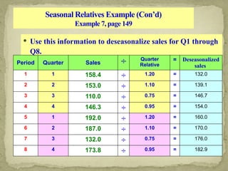
This document discusses forecasting techniques used to predict future values of variables like demand and resource availability. It outlines key forecasting aspects such as accuracy, method selection, and the importance of trends and seasonality, as well as various qualitative and quantitative approaches. Additionally, it provides formulas and examples for error calculation, moving averages, and seasonal adjustments, emphasizing the need for timely, accurate, and reliable forecasts.

1. Forecasting
Chapter 3
McGraw-Hill/Irwin
Copyright © 2012 by The McGraw-Hill Companies, Inc. All rights reserved.

2. Forecast
 Forecast – a statement about the future value
of a variable of interest
 We make forecasts about such things as weather,
demand, and resource availability
 Forecasts are an important element in making
informed decisions
Instructor Slides 3-2

3. Two Important Aspects of Forecasts
 Expected level of demand
 The level of demand may be a function of some
structural variation such as trend or seasonal
variation
 Accuracy
 Related to the potential size of forecast error
Instructor Slides 3-3

4. Elements of a Good Forecast
The forecast
 should be timely
 should be accurate
 should be reliable
 should be expressed in meaningful units
 should be in writing
 technique should be simple to understand and
use
 should be cost effective

5. Steps in the Forecasting Process
1. Determine the purpose of the forecast
2. Establish a time horizon
3. Select a forecasting technique
4. Obtain, clean, and analyze appropriate data
5. Make the forecast
6. Monitor the forecast

6. Features Common to All Forecasts
1. Techniques assume some underlying causal
system that existed in the past will persist into the
future
2. Forecasts are not perfect
3. Forecasts for groups of items are more accurate
than those for individual items
4. Forecast accuracy decreases as the forecasting
horizon increases
Instructor Slides 3-6

7. Forecast Accuracy and Control
Forecast errors should be
monitored
 Error = Actual – Forecast
 If errors fall beyond acceptable bounds,
corrective action may be necessary

8. Forecast Accuracy Metrics
n
 

t
t Forecast
Actual
MAD
 2
t
t
1
Forecast
Actual
MSE




n
100
Actual
Forecast
Actual
MAPE
t
t
t





n
MAD weights all errors
evenly
MSE weights errors according
to their squared values
MAPE weights errors
according to relative error

9. Forecast Error Calculation
Period
Actual
(A)
Forecast
(F)
(A-F)
Error |Error| Error2
1 107 110 -3 3 9
2 125 121 4 4 16
3 115 112 3 3 9
4 118 120 -2 2 4
5 108 109 -1 1 1
AVG(A) 114.6
Sum 13 39
n = 5 n-1 = 4
MAD MSE MAPE=MAD / AVG(A)
= 2.6 = 9.75 =2.6/114.6= 2.27%

10. Forecasting Approaches
 Qualitative Forecasting
 Qualitative techniques permit the inclusion of soft information
such as:
 Human factors
 Personal opinions
 Hunches
 These factors are difficult, or impossible, to quantify
 Quantitative Forecasting
 Quantitative techniques involve either the projection of historical
data or the development of associative methods that attempt to use
causal variables to make a forecast
 These techniques rely on hard data

11. Judgmental Forecasts
 Forecasts that use subjective inputs such as
opinions from consumer surveys, sales staff,
managers, executives, and experts
 Executive opinions
 Sales force opinions
 Consumer surveys
 Delphi method

12. Time-Series Forecasts
 Forecasts that project patterns identified in
recent time-series observations
 Time-series - a time-ordered sequence of
observations taken at regular time intervals
 Assume that future values of the time-series
can be estimated from past values of the time-
series

13. Time-Series Behaviors
 Trend
 Seasonality
 Cycles
 Irregular variations
 Random variation

14. Historical Monthly Product Demand Consisting of a
Growth Trend, Cyclical Factor, and Seasonal Demand
Exhibit 9.4

15. Common Types of Trends
Exhibit 9.5a

16. Common Types of Trends (cont’d)
Exhibit 9.5b

17. Trends and Seasonality
 Trend
 A long-term upward or downward movement in data
 Population shifts
 Changing income
 Seasonality
 Short-term, fairly regular variations related to the calendar
or time of day
 Restaurants, service call centers, and theaters all experience
seasonal demand

18. Trend, Cyclical, with Variations

19. Cycles and Variations
 Cycle
 Wavelike variations lasting more than one year
 These are often related to a variety of economic, political, or
even agricultural conditions
 Random Variation
 Residual variation that remains after all other behaviors
have been accounted for
 Irregular variation
 Due to unusual circumstances that do not reflect typical
behavior
 Labor strike
 Weather event

20. Time-Series Forecasting - Naïve Forecast
 Naïve Forecast
 Uses a single previous value of a time series as the
basis for a forecast
 The forecast for a time period is equal to the
previous time period’s value
 Can be used when
 The time series is stable
 There is a trend
 There is seasonality

21. Time-Series Forecasting - Averaging
 These Techniques work best when a series
tends to vary about an average
 Averaging techniques smooth variations in the
data
 They can handle step changes or gradual changes
in the level of a series
 Techniques
 Moving average
 Weighted moving average
 Exponential smoothing

22. Moving Average
 Technique that averages a number of the most
recent actual values in generating a forecast
average
moving
in the
periods
of
Number
1
period
in
value
Actual
average
moving
period
MA
period
for time
Forecast
where
MA
1
1
t











n
t
A
n
t
F
n
A
F
t
t
t
n
i
i
t
t

23. Forecast Demand Based on aThree- and
Five-Week Simple MovingAverage
Week Demand Forecast Forecast
(3-week) (5-week)
1 800
2 1400
3 1000
4 1500 (1000+1400+800)/3 =1067
5 1500 (1500+1000+1400)/3 = 1300
6 1300 (1500+1500+1000)/3 = 1333 (1500+1500+1000+1400+ 800)/5 =1240
7 1800 (1300+1500+1500)/3 = 1433 (1300+1500+1500+1000+1400)/5 =1340
8 1700 (1800+1300+1500)/3 = 1533 (1800+1300+1500+1500+1000)/5 =1420
9 1300 1600 (1700+1800+1300+1500+1500)/5 =1560
10 1700 1600 (1300+1700+1800+1300+1500)/5 =1520
11 1700 1567 (1700+1300+1700+1800+1300)/5 =1560

24. Moving Average
 As new data become available, the forecast is
updated by adding the newest value and
dropping the oldest and then recomputing the
the average
 The number of data points included in the
average determines the model’s sensitivity
 Fewer data points used-- more responsive
 More data points used-- less responsive

25. Forecast Demand Based on a Three- and
Nine-Week Simple Moving Average
Exhibit 9.6

26. MovingAverage Forecast ofThree- and
Nine-Week Periods versusActual Demand
Exhibit 9.7

27. Weighted Moving Average
 The most recent values in a time series are
given more weight in computing a forecast
 The choice of weights, w, is somewhat arbitrary
and involves some trial and error

Ft wn At n  wn 1At (n 1)  ... w1At 1
where
wt weight for period t, wt 1 weight for period t  1, etc.
At the actual value for period t, At 1 the actual value for period t  1, etc.

28. Exponential Smoothing
 A weighted averaging method that is based on
the previous forecast plus a percentage of the
forecast error
1 1 1
1
1
( )
where
Forecast for period
Forecast for the previous period
=Smoothing constant
Actual demand or sales from the previous period
t t t t
t
t
t
F F A F
F t
F
A


  


  




29. Exponential Smoothing
Saturday Hotel Occupancy ( =0.5)
Forecast
Period Occupancy Forecast Error
t At Ft |At - Ft|
1 79 ---
2 84 79.00 5
3 83 79+.5(84-79)=81.50 or 82 1
4 81 81.5+.5(83-81.5)=82.25 or 82 1
5 98 82.25+.5(81-82.25)=81.63 or 82 16
6 100 81.63+.5(98-81.63)= 89.81 or 90 10
MAD =33/5= 6.6
Forecast Error (Mean Absolute Deviation) = ΣlAt – Ftl / n
The first actual value as the forecast for period 2

17-29

30. Linear Trend
 A simple data plot can reveal the existence
and nature of a trend
 Linear trend equation
Ft a  bt
where
Ft Forecast for period t
a Value of Ft at t 0
b Slope of the line
t Specified number of time periods from t 0

31. Estimating slope and intercept
 Slope and intercept can be estimated from
historical data
 
2
2
or
where
Number of periods
Value of the time series
n ty t y
b
n t t
y b t
a y bt
n
n
y




 


  
 
 

32. Figure 3-9
3-32

33. Linear Trend Example
Week (t) Sales (y) t2
ty
1 150 1 150
2 157 4 314
3 162 9 486
4 166 16 664
5 177 25 885
t= 15 y= 812 t2
=55 (ty)=2499

34. Linear Trend Example
 
2
2
5(2499) 15(812)
5(55) 225
12495 12180
6.3
275 225
812-6.3(15)
= 143.5
5
143.5 6.3
n ty t y
b
n t t
y b t
a
n
y t
 
 



 


 
 
  
 
 

35. Linear Trend Example
Substituting values of t into this
equation, the forecast for next 2
periods are:
F6= 143.5+6.3 (6) = 181.3
F7= 143.5+6.3 (7) = 187.6

36. Techniques for Seasonality
 Seasonality – regularly repeating movements in
series values that can be tied to recurring events
 Expressed in terms of the amount that actual values
deviate from the average value of a series
 Models of seasonality
 Additive
 Seasonality is expressed as a quantity that gets added to or
subtracted from the time-series average in order to
incorporate seasonality
 Multiplicative
 Seasonality is expressed as a percentage of the average (or
trend) amount which is then used to multiply the value of a
series in order to incorporate seasonality
Instructor Slides 3-36

37. Models of Seasonality
Instructor Slides 3-37

38. Computing Seasonal Relatives Using SimpleAverage (SA) Method
Example 8A, page 150
 Manager of a Call center recorded the volume of calls received
between 9 and 10 a.m. for 21 days and wants to obtain a seasonal
index for each day for that hour.
Volume Season Overall
Day Week 1 Week 2 Week 3 Average ÷ Average = SA Index
Tues 67 60 64 63.667 ÷ 71.571 = 0.8896
Wed 75 73 76 74.667 ÷ 71.571 = 1.0432
Thurs 82 85 87 84.667 ÷ 71.571 = 1.1830
Fri 98 99 96 97.667 ÷ 71.571 = 1.3646
Sat 90 86 88 88.000 ÷ 71.571 = 1.2295
Sun 36 40 44 40.000 ÷ 71.571 = 0.5589
Mon 55 52 50 52.333 ÷ 71.571 = 0.7312
Overall Avg 71.571 7.0000

39. Seasonal Relatives
 Seasonal relatives
 The seasonal percentage used in the multiplicative
seasonally adjusted forecasting model
 Using seasonal relatives
 To deseasonalize data
 Done in order to get a clearer picture of the nonseasonal
components of the data series
 Divide each data point by its seasonal relative
 To incorporate seasonality in a forecast
 Obtain trend estimates for desired periods using a trend
equation
 Add seasonality by multiplying these trend estimates
by the corresponding seasonal relative

40. Seasonal Relatives Example
Example 7, page 149
 A coffee shop owner wants to predict quarterly
demand for hot chocolate for periods 9 and 10, which
happen to be the 1st
and 2nd
quarters of a particular
year. The sales data consist of both trend and
seasonality. The trend portion of demand is projected
using the equation Ft = 124 + 7.5 t. Quarter relatives
are
Q1 = 1.20, Q2 = 1.10, Q3 = 0.75, Q4 = 0.95,

41. Seasonal Relatives Example (Con’d)
Example 7, page 149
 Use this information to deseasonalize sales for Q1 through
Q8.
Period Quarter Sales ÷ Quarter
Relative
= Deseasonalized
sales
1 1 158.4 ÷ 1.20 = 132.0
2 2 153.0 ÷ 1.10 = 139.1
3 3 110.0 ÷ 0.75 = 146.7
4 4 146.3 ÷ 0.95 = 154.0
5 1 192.0 ÷ 1.20 = 160.0
6 2 187.0 ÷ 1.10 = 170.0
7 3 132.0 ÷ 0.75 = 176.0
8 4 173.8 ÷ 0.95 = 182.9

42. Seasonal Relatives Example (Con’d)
Example 7, page 149
 Use this information to predict for periods 9 and 10.
 F9 = 124 +7.5( 9) = 191.5
F10= 124 +7.5(10) = 199.0
Multiplying the trend value by the appropriate quarter
relative yields a forecast that includes both trend and
seasonality.
Given that t =9 is a 1st
quarter and t = 10 is a 2nd
quarter.
The forecast demand for period 9 = 191.5(1.20) = 229.8
The forecast demand for period 10 = 199.0(1.10) = 218.9