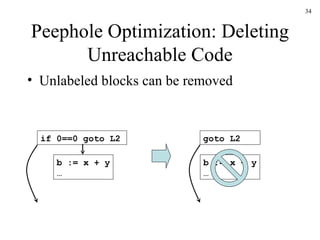
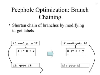
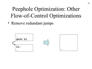
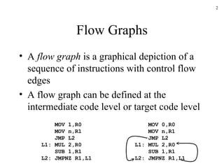
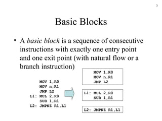
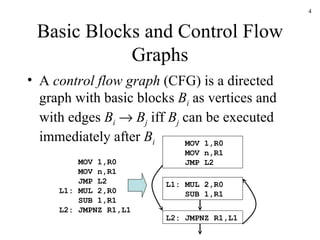
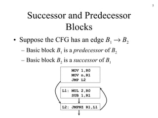
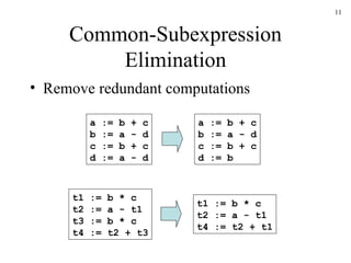
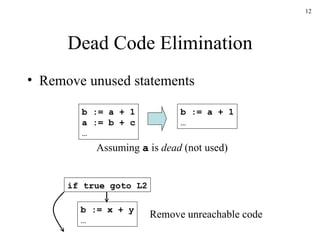
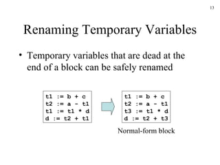
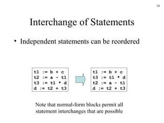
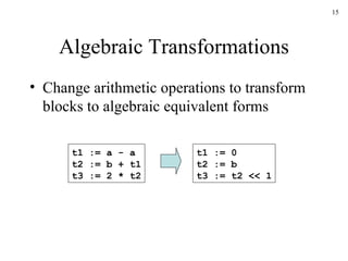
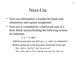
Code Generation Part II Chapter 8 (1 st  ed. Ch.9) COP5621 Compiler Construction Copyright Robert van Engelen, Florida State University, 2007-2009
Flow Graphs A  flow graph  is a graphical depiction of a sequence of instructions with control flow edges A flow graph can be defined at the intermediate code level or target code level MOV 1,R0   MOV n,R1   JMP L2 L1: MUL 2,R0   SUB 1,R1 L2: JMPNZ R1,L1 MOV 0,R0   MOV n,R1   JMP L2 L1: MUL 2,R0   SUB 1,R1 L2: JMPNZ R1,L1
Basic Blocks A  basic block  is a sequence of consecutive instructions with exactly one entry point and one exit point (with natural flow or a branch instruction) MOV 1,R0   MOV n,R1   JMP L2 MOV 1,R0   MOV n,R1   JMP L2 L1: MUL 2,R0   SUB 1,R1 L2: JMPNZ R1,L1 L1: MUL 2,R0   SUB 1,R1 L2: JMPNZ R1,L1
Basic Blocks and Control Flow Graphs A  control flow graph  (CFG) is a directed graph with basic blocks  B i  as vertices and with edges  B i      B j  iff  B j  can be executed immediately after  B i MOV 1,R0   MOV n,R1   JMP L2 MOV 1,R0   MOV n,R1   JMP L2 L1: MUL 2,R0   SUB 1,R1 L2: JMPNZ R1,L1 L1: MUL 2,R0   SUB 1,R1 L2: JMPNZ R1,L1
Successor and Predecessor Blocks Suppose the CFG has an edge  B 1      B 2 Basic block  B 1  is a  predecessor  of  B 2   Basic block  B 2  is a  successor  of  B 1 MOV 1,R0   MOV n,R1   JMP L2 L1: MUL 2,R0   SUB 1,R1 L2: JMPNZ R1,L1
Partition Algorithm for Basic Blocks Input : A sequence of three-address statements Output : A list of basic blocks with each three-address statement  in exactly one block Determine the set of  leaders , the first statements if basic blocks The first statement is the leader Any statement that is the target of a goto is a leader Any statement that immediately follows a goto is a leader For each leader, its basic block consist of the leader and all statements up to but not including the next leader or the end of the program
Loops A  loop  is a collection of basic blocks, such that All blocks in the collection are  strongly connected The collection has a unique  entry , and the only way to reach a block in the loop is through the entry
Loops (Example) MOV 1,R0   MOV n,R1   JMP L2 L1: MUL 2,R0   SUB 1,R1 L2: JMPNZ R1,L1 B1: B2: B3: L3: ADD 2,R2   SUB 1,R0   JMPNZ R0,L3 B4: Strongly connected components: SCC={ {B2,B3}, {B4} } Entries: B3, B4
Equivalence of Basic Blocks Two basic blocks are (semantically)  equivalent  if they compute the same set of expressions b  := 0 t1 := a + b t2 := c * t1 a  := t2 a  := c * a b  := 0 a := c*a b := 0 a := c*a b := 0 Blocks are equivalent, assuming  t1  and  t2  are  dead : no longer used (no longer  live )
Transformations on Basic Blocks A  code-improving transformation  is a code optimization to improve speed or reduce code size Global transformations  are performed across basic blocks Local transformations  are only performed on single basic blocks Transformations must be safe and preserve the meaning of the code A local transformation is safe if the transformed basic block is guaranteed to be equivalent to its original form
Common-Subexpression Elimination Remove redundant computations a := b + c b := a - d c := b + c d := a - d a := b + c b := a - d c := b + c d := b t1 := b * c t2 := a - t1 t3 := b * c t4 := t2 + t3 t1 := b * c t2 := a - t1 t4 := t2 + t1
Dead Code Elimination Remove unused statements b := a + 1 a := b + c … b := a + 1 … Assuming  a  is  dead  (not used) b := x + y … if true goto L2 Remove unreachable code
Renaming Temporary Variables Temporary variables that are dead at the end of a block can be safely renamed t1 := b + c t2 := a - t1 t1 := t1 * d d := t2 + t1 t1 := b + c t2 := a - t1 t3 := t1 * d d := t2 + t3 Normal-form block
Interchange of Statements Independent statements can be reordered t1 := b + c t2 := a - t1 t3 := t1 * d d := t2 + t3 t1 := b + c t3 := t1 * d t2 := a - t1 d := t2 + t3 Note that normal-form blocks permit all statement interchanges that are possible
Algebraic Transformations Change arithmetic operations to transform blocks to algebraic equivalent forms t1 := a - a t2 := b + t1 t3 := 2 * t2 t1 := 0 t2 := b t3 := t2 << 1
Next-Use Next-use information is needed for dead-code elimination and register assignment Next-use is computed by a backward scan of a basic block and performing the following actions on statement i :  x  :=  y  op  z Add liveness/next-use info on  x ,  y , and  z  to statement  i Before going up to the previous statement (scan up): Set  x  info to “not live” and “no next use” Set  y  and  z  info to “live” and the next uses of  y  and  z  to  i
Next-Use (Step 1) i :  a := b + c j :  t := a + b [  live ( a ) = true,  live ( b ) = true,  live ( t ) = true,   nextuse ( a ) = none,  nextuse ( b ) = none,  nextuse ( t ) = none ] Attach current live/next-use information Because info is empty, assume variables are live (Data flow analysis Ch.10 can provide accurate information)
Next-Use (Step 2) i :  a := b + c j :  t := a + b [  live ( a ) = true,  live ( b ) = true,  live ( t ) = true,   nextuse ( a ) = none,  nextuse ( b ) = none,  nextuse ( t ) = none ] live ( a ) = true nextuse ( a ) =  j live ( b ) = true nextuse ( b ) =  j live ( t ) = false nextuse ( t ) = none Compute live/next-use information at  j
Next-Use (Step 3) i :  a := b + c j :  t := a + b [  live ( a ) = true,  live ( b ) = true,  live ( t ) = true,   nextuse ( a ) = none,  nextuse ( b ) = none,  nextuse ( t ) = none ] Attach current live/next-use information to  i [  live ( a ) = true,  live ( b ) = true,  live ( c ) = false,   nextuse ( a ) =  j ,  nextuse ( b ) =  j ,  nextuse ( c ) = none ]
Next-Use (Step 4) i :  a := b + c j :  t := a + b live ( a ) = false nextuse ( a ) = none live ( b ) = true nextuse ( b ) =  i live ( c ) = true nextuse ( c ) =  i live ( t ) = false nextuse ( t ) = none [  live ( a ) = false,  live ( b ) = false,  live ( t ) = false,   nextuse ( a ) = none,  nextuse ( b ) = none,  nextuse ( t ) = none ] [  live ( a ) = true,  live ( b ) = true,  live ( c ) = false,   nextuse ( a ) =  j ,  nextuse ( b ) =  j ,  nextuse ( c ) = none ] Compute live/next-use information  i
A Code Generator Generates target code for a sequence of three-address statements using next-use information Uses new function  getreg  to assign registers to variables Computed results are kept in registers as long as possible, which means: Result is needed in another computation Register is kept up to a procedure call or end of block Checks if operands to three-address code are available in registers
The Code Generation Algorithm For each statement  x  :=  y  op  z Set location  L  =  getreg ( y ,  z ) If  y      L  then generate MOV   y’ , L where  y’  denotes one of the locations where the value of  y  is available (choose register if possible) Generate OP   z’ , L where  z’  is one of the locations of  z ; Update register/address descriptor of  x  to include  L If  y  and/or  z  has no next use and is stored in register, update register descriptors to remove  y  and/or  z
Register and Address Descriptors A  register descriptor  keeps track of what is currently stored in a register at a particular point in the code, e.g. a local variable, argument, global variable, etc. MOV a,R0 “ R0  contains  a ” An  address descriptor  keeps track of the location where the current value of the name can be found at run time, e.g. a register, stack location, memory address, etc. MOV a,R0 MOV R0,R1 “ a  in  R0  and  R1 ”
The  getreg  Algorithm To compute  getreg ( y , z ) If  y  is stored in a register  R  and  R  only holds the value  y , and  y  has no next use, then return  R ; Update address descriptor: value  y  no longer in  R Else, return a new empty register if available Else, find an occupied register  R ; Store contents (register spill) by generating MOV  R , M for every  M  in address descriptor of  y ; Return register  R Return a memory location
Code Generation Example Statements Code Generated Register Descriptor Address Descriptor t := a - b u := a - c v := t + u d := v + u MOV a,R0 SUB b,R0 MOV a,R1 SUB c,R1 ADD R1,R0 ADD R1,R0 MOV R0,d Registers empty R0  contains  t R0  contains  t R1  contains  u R0  contains  v R1  contains  u R0  contains  d t  in  R0 t  in  R0 u  in  R1 u  in  R1 v  in  R0 d  in  R0 d  in  R0  and memory
Register Allocation and Assignment The  getreg  algorithm is simple but sub-optimal All live variables in registers are stored (flushed) at the end of a block Global register allocation  assigns variables to limited number of available registers and attempts to keep these registers consistent across basic block boundaries Keeping variables in registers in looping code can result in big savings
Allocating Registers in Loops Suppose loading a variable  x  has a cost of 2 Suppose storing a variable  x  has a cost of 2 Benefit of allocating a register to a variable  x  within a loop  L  is  B  L  (  use ( x ,  B ) + 2  live ( x ,  B ) ) where  use ( x ,  B ) is the number of times  x  is used in  B  and  live ( x ,  B ) = true if  x  is live on exit from  B
Global Register Allocation with Graph Coloring When a register is needed but all available registers are in use, the content of one of the used registers must be stored (spilled) to free a register Graph coloring allocates registers and attempts to minimize the cost of spills Build a  conflict graph  ( interference graph ) Find a  k -coloring for the graph, with  k  the number of registers
Register Allocation with Graph Coloring: Example a := read(); b := read(); c := read(); a := a + b + c; if (a < 10) {   d := c + 8;   write(c); } else if (a < 20) {   e := 10;   d := e + a;   write(e); } else {   f := 12;   d := f + a;   write(f); } write(d);
Register Allocation with Graph Coloring: Live Ranges a := read(); b := read(); c := read(); a := a+b+c; a < 20 a < 10 d := c+8; write(c); f := 12; d := f+a; write(f); e := 10; d := e+a; write(e); write(d); a b c e f d d d a f b d e c Interference graph : connected vars have overlapping ranges Live range of  b
Register Allocation with Graph Coloring: Solution a f b d e c Interference graph 2 1 3 2 1 1 Solve Three registers: a = r2 b = r3 c = r1 d = r2 e = r1 f = r1 r2 := read(); r3 := read(); r1 := read(); r2 := r2 + r3 + r1; if (r2 < 10) {   r2 := r1 + 8;   write(r1); } else if (r2 < 20) {   r1 := 10;   r2 := r1 + r2;   write(r1); } else {   r1 := 12;   r2 := r1 + r2;   write(r1); } write(r2);
Peephole Optimization Examines a short sequence of target instructions in a window ( peephole ) and replaces the instructions by a faster and/or shorter sequence when possible Applied to intermediate code or target code Typical optimizations: Redundant instruction elimination Flow-of-control optimizations Algebraic simplifications Use of machine idioms
Peephole Opt: Eliminating Redundant Loads and Stores Consider MOV R0,a MOV a,R0 The second instruction can be deleted, but only if it is not labeled with a target label Peephole represents sequence of instructions with at most one entry point The first instruction can also be deleted if  live ( a )=false
Peephole Optimization: Deleting Unreachable Code Unlabeled blocks can be removed b := x + y … goto L2 b := x + y … if 0==0 goto L2
Peephole Optimization: Branch Chaining Shorten chain of branches by modifying target labels b := x + y … if a==0 goto L2 L2: goto L3 b := x + y … if a==0 goto L3 L2: goto L3
Peephole Optimization: Other Flow-of-Control Optimizations Remove redundant jumps L1: … … goto L1 …
Other Peephole Optimizations Reduction in strength : replace expensive arithmetic operations with cheaper ones Utilize machine idioms Algebraic simplifications … a := x ^ 2 b := y / 8 … a := x * x b := y >> 3 … a := a + 1 … inc a … a := a + 0 b := b * 1 …

Ch9b

  • 1.
    Code Generation PartII Chapter 8 (1 st ed. Ch.9) COP5621 Compiler Construction Copyright Robert van Engelen, Florida State University, 2007-2009
  • 2.
    Flow Graphs A flow graph is a graphical depiction of a sequence of instructions with control flow edges A flow graph can be defined at the intermediate code level or target code level MOV 1,R0 MOV n,R1 JMP L2 L1: MUL 2,R0 SUB 1,R1 L2: JMPNZ R1,L1 MOV 0,R0 MOV n,R1 JMP L2 L1: MUL 2,R0 SUB 1,R1 L2: JMPNZ R1,L1
  • 3.
    Basic Blocks A basic block is a sequence of consecutive instructions with exactly one entry point and one exit point (with natural flow or a branch instruction) MOV 1,R0 MOV n,R1 JMP L2 MOV 1,R0 MOV n,R1 JMP L2 L1: MUL 2,R0 SUB 1,R1 L2: JMPNZ R1,L1 L1: MUL 2,R0 SUB 1,R1 L2: JMPNZ R1,L1
  • 4.
    Basic Blocks andControl Flow Graphs A control flow graph (CFG) is a directed graph with basic blocks B i as vertices and with edges B i  B j iff B j can be executed immediately after B i MOV 1,R0 MOV n,R1 JMP L2 MOV 1,R0 MOV n,R1 JMP L2 L1: MUL 2,R0 SUB 1,R1 L2: JMPNZ R1,L1 L1: MUL 2,R0 SUB 1,R1 L2: JMPNZ R1,L1
  • 5.
    Successor and PredecessorBlocks Suppose the CFG has an edge B 1  B 2 Basic block B 1 is a predecessor of B 2 Basic block B 2 is a successor of B 1 MOV 1,R0 MOV n,R1 JMP L2 L1: MUL 2,R0 SUB 1,R1 L2: JMPNZ R1,L1
  • 6.
    Partition Algorithm forBasic Blocks Input : A sequence of three-address statements Output : A list of basic blocks with each three-address statement in exactly one block Determine the set of leaders , the first statements if basic blocks The first statement is the leader Any statement that is the target of a goto is a leader Any statement that immediately follows a goto is a leader For each leader, its basic block consist of the leader and all statements up to but not including the next leader or the end of the program
  • 7.
    Loops A loop is a collection of basic blocks, such that All blocks in the collection are strongly connected The collection has a unique entry , and the only way to reach a block in the loop is through the entry
  • 8.
    Loops (Example) MOV1,R0 MOV n,R1 JMP L2 L1: MUL 2,R0 SUB 1,R1 L2: JMPNZ R1,L1 B1: B2: B3: L3: ADD 2,R2 SUB 1,R0 JMPNZ R0,L3 B4: Strongly connected components: SCC={ {B2,B3}, {B4} } Entries: B3, B4
  • 9.
    Equivalence of BasicBlocks Two basic blocks are (semantically) equivalent if they compute the same set of expressions b := 0 t1 := a + b t2 := c * t1 a := t2 a := c * a b := 0 a := c*a b := 0 a := c*a b := 0 Blocks are equivalent, assuming t1 and t2 are dead : no longer used (no longer live )
  • 10.
    Transformations on BasicBlocks A code-improving transformation is a code optimization to improve speed or reduce code size Global transformations are performed across basic blocks Local transformations are only performed on single basic blocks Transformations must be safe and preserve the meaning of the code A local transformation is safe if the transformed basic block is guaranteed to be equivalent to its original form
  • 11.
    Common-Subexpression Elimination Removeredundant computations a := b + c b := a - d c := b + c d := a - d a := b + c b := a - d c := b + c d := b t1 := b * c t2 := a - t1 t3 := b * c t4 := t2 + t3 t1 := b * c t2 := a - t1 t4 := t2 + t1
  • 12.
    Dead Code EliminationRemove unused statements b := a + 1 a := b + c … b := a + 1 … Assuming a is dead (not used) b := x + y … if true goto L2 Remove unreachable code
  • 13.
    Renaming Temporary VariablesTemporary variables that are dead at the end of a block can be safely renamed t1 := b + c t2 := a - t1 t1 := t1 * d d := t2 + t1 t1 := b + c t2 := a - t1 t3 := t1 * d d := t2 + t3 Normal-form block
  • 14.
    Interchange of StatementsIndependent statements can be reordered t1 := b + c t2 := a - t1 t3 := t1 * d d := t2 + t3 t1 := b + c t3 := t1 * d t2 := a - t1 d := t2 + t3 Note that normal-form blocks permit all statement interchanges that are possible
  • 15.
    Algebraic Transformations Changearithmetic operations to transform blocks to algebraic equivalent forms t1 := a - a t2 := b + t1 t3 := 2 * t2 t1 := 0 t2 := b t3 := t2 << 1
  • 16.
    Next-Use Next-use informationis needed for dead-code elimination and register assignment Next-use is computed by a backward scan of a basic block and performing the following actions on statement i : x := y op z Add liveness/next-use info on x , y , and z to statement i Before going up to the previous statement (scan up): Set x info to “not live” and “no next use” Set y and z info to “live” and the next uses of y and z to i
  • 17.
    Next-Use (Step 1)i : a := b + c j : t := a + b [ live ( a ) = true, live ( b ) = true, live ( t ) = true, nextuse ( a ) = none, nextuse ( b ) = none, nextuse ( t ) = none ] Attach current live/next-use information Because info is empty, assume variables are live (Data flow analysis Ch.10 can provide accurate information)
  • 18.
    Next-Use (Step 2)i : a := b + c j : t := a + b [ live ( a ) = true, live ( b ) = true, live ( t ) = true, nextuse ( a ) = none, nextuse ( b ) = none, nextuse ( t ) = none ] live ( a ) = true nextuse ( a ) = j live ( b ) = true nextuse ( b ) = j live ( t ) = false nextuse ( t ) = none Compute live/next-use information at j
  • 19.
    Next-Use (Step 3)i : a := b + c j : t := a + b [ live ( a ) = true, live ( b ) = true, live ( t ) = true, nextuse ( a ) = none, nextuse ( b ) = none, nextuse ( t ) = none ] Attach current live/next-use information to i [ live ( a ) = true, live ( b ) = true, live ( c ) = false, nextuse ( a ) = j , nextuse ( b ) = j , nextuse ( c ) = none ]
  • 20.
    Next-Use (Step 4)i : a := b + c j : t := a + b live ( a ) = false nextuse ( a ) = none live ( b ) = true nextuse ( b ) = i live ( c ) = true nextuse ( c ) = i live ( t ) = false nextuse ( t ) = none [ live ( a ) = false, live ( b ) = false, live ( t ) = false, nextuse ( a ) = none, nextuse ( b ) = none, nextuse ( t ) = none ] [ live ( a ) = true, live ( b ) = true, live ( c ) = false, nextuse ( a ) = j , nextuse ( b ) = j , nextuse ( c ) = none ] Compute live/next-use information i
  • 21.
    A Code GeneratorGenerates target code for a sequence of three-address statements using next-use information Uses new function getreg to assign registers to variables Computed results are kept in registers as long as possible, which means: Result is needed in another computation Register is kept up to a procedure call or end of block Checks if operands to three-address code are available in registers
  • 22.
    The Code GenerationAlgorithm For each statement x := y op z Set location L = getreg ( y , z ) If y  L then generate MOV y’ , L where y’ denotes one of the locations where the value of y is available (choose register if possible) Generate OP z’ , L where z’ is one of the locations of z ; Update register/address descriptor of x to include L If y and/or z has no next use and is stored in register, update register descriptors to remove y and/or z
  • 23.
    Register and AddressDescriptors A register descriptor keeps track of what is currently stored in a register at a particular point in the code, e.g. a local variable, argument, global variable, etc. MOV a,R0 “ R0 contains a ” An address descriptor keeps track of the location where the current value of the name can be found at run time, e.g. a register, stack location, memory address, etc. MOV a,R0 MOV R0,R1 “ a in R0 and R1 ”
  • 24.
    The getreg Algorithm To compute getreg ( y , z ) If y is stored in a register R and R only holds the value y , and y has no next use, then return R ; Update address descriptor: value y no longer in R Else, return a new empty register if available Else, find an occupied register R ; Store contents (register spill) by generating MOV R , M for every M in address descriptor of y ; Return register R Return a memory location
  • 25.
    Code Generation ExampleStatements Code Generated Register Descriptor Address Descriptor t := a - b u := a - c v := t + u d := v + u MOV a,R0 SUB b,R0 MOV a,R1 SUB c,R1 ADD R1,R0 ADD R1,R0 MOV R0,d Registers empty R0 contains t R0 contains t R1 contains u R0 contains v R1 contains u R0 contains d t in R0 t in R0 u in R1 u in R1 v in R0 d in R0 d in R0 and memory
  • 26.
    Register Allocation andAssignment The getreg algorithm is simple but sub-optimal All live variables in registers are stored (flushed) at the end of a block Global register allocation assigns variables to limited number of available registers and attempts to keep these registers consistent across basic block boundaries Keeping variables in registers in looping code can result in big savings
  • 27.
    Allocating Registers inLoops Suppose loading a variable x has a cost of 2 Suppose storing a variable x has a cost of 2 Benefit of allocating a register to a variable x within a loop L is  B  L ( use ( x , B ) + 2 live ( x , B ) ) where use ( x , B ) is the number of times x is used in B and live ( x , B ) = true if x is live on exit from B
  • 28.
    Global Register Allocationwith Graph Coloring When a register is needed but all available registers are in use, the content of one of the used registers must be stored (spilled) to free a register Graph coloring allocates registers and attempts to minimize the cost of spills Build a conflict graph ( interference graph ) Find a k -coloring for the graph, with k the number of registers
  • 29.
    Register Allocation withGraph Coloring: Example a := read(); b := read(); c := read(); a := a + b + c; if (a < 10) { d := c + 8; write(c); } else if (a < 20) { e := 10; d := e + a; write(e); } else { f := 12; d := f + a; write(f); } write(d);
  • 30.
    Register Allocation withGraph Coloring: Live Ranges a := read(); b := read(); c := read(); a := a+b+c; a < 20 a < 10 d := c+8; write(c); f := 12; d := f+a; write(f); e := 10; d := e+a; write(e); write(d); a b c e f d d d a f b d e c Interference graph : connected vars have overlapping ranges Live range of b
  • 31.
    Register Allocation withGraph Coloring: Solution a f b d e c Interference graph 2 1 3 2 1 1 Solve Three registers: a = r2 b = r3 c = r1 d = r2 e = r1 f = r1 r2 := read(); r3 := read(); r1 := read(); r2 := r2 + r3 + r1; if (r2 < 10) { r2 := r1 + 8; write(r1); } else if (r2 < 20) { r1 := 10; r2 := r1 + r2; write(r1); } else { r1 := 12; r2 := r1 + r2; write(r1); } write(r2);
  • 32.
    Peephole Optimization Examinesa short sequence of target instructions in a window ( peephole ) and replaces the instructions by a faster and/or shorter sequence when possible Applied to intermediate code or target code Typical optimizations: Redundant instruction elimination Flow-of-control optimizations Algebraic simplifications Use of machine idioms
  • 33.
    Peephole Opt: EliminatingRedundant Loads and Stores Consider MOV R0,a MOV a,R0 The second instruction can be deleted, but only if it is not labeled with a target label Peephole represents sequence of instructions with at most one entry point The first instruction can also be deleted if live ( a )=false
  • 34.
    Peephole Optimization: DeletingUnreachable Code Unlabeled blocks can be removed b := x + y … goto L2 b := x + y … if 0==0 goto L2
  • 35.
    Peephole Optimization: BranchChaining Shorten chain of branches by modifying target labels b := x + y … if a==0 goto L2 L2: goto L3 b := x + y … if a==0 goto L3 L2: goto L3
  • 36.
    Peephole Optimization: OtherFlow-of-Control Optimizations Remove redundant jumps L1: … … goto L1 …
  • 37.
    Other Peephole OptimizationsReduction in strength : replace expensive arithmetic operations with cheaper ones Utilize machine idioms Algebraic simplifications … a := x ^ 2 b := y / 8 … a := x * x b := y >> 3 … a := a + 1 … inc a … a := a + 0 b := b * 1 …