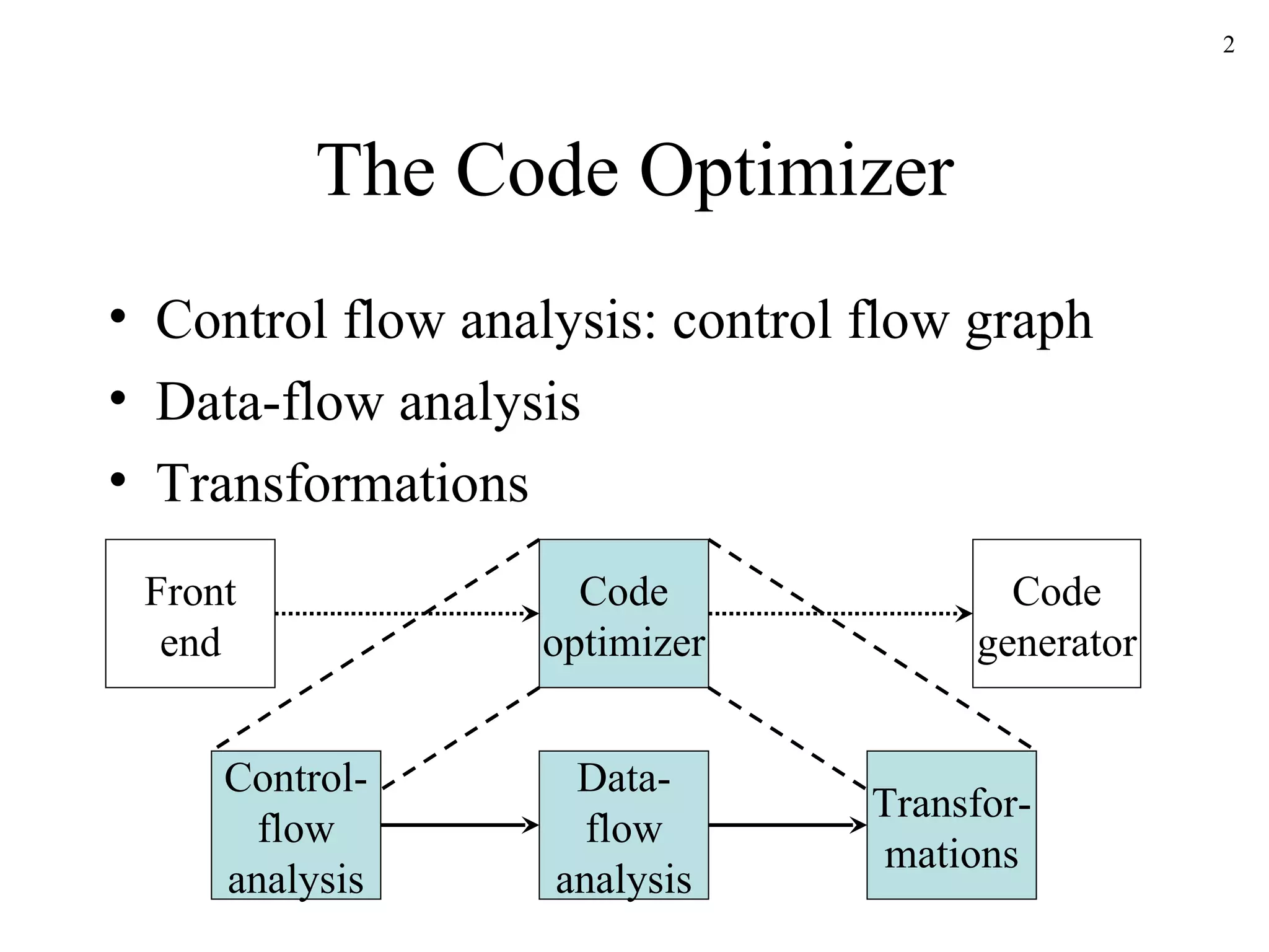
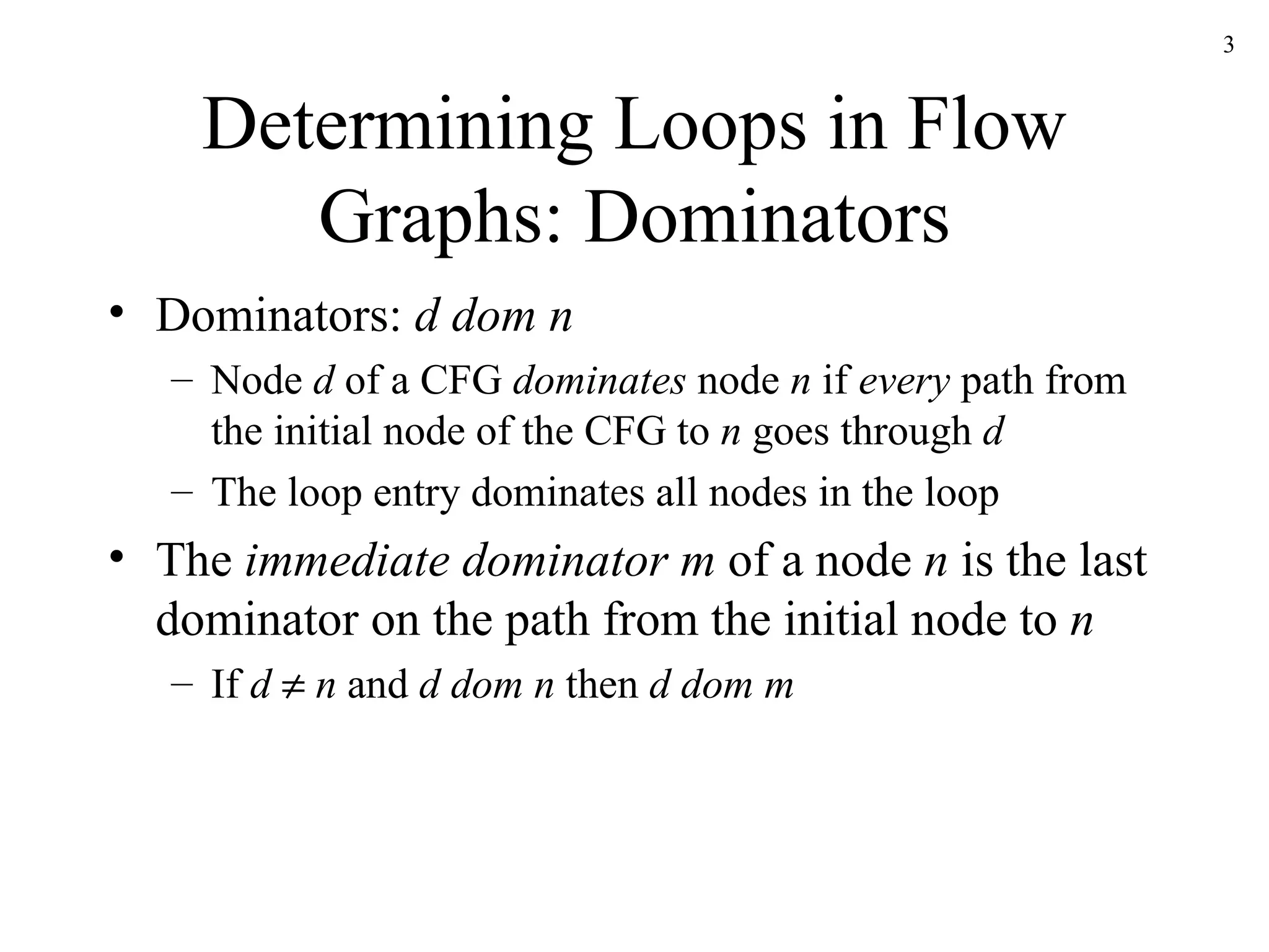
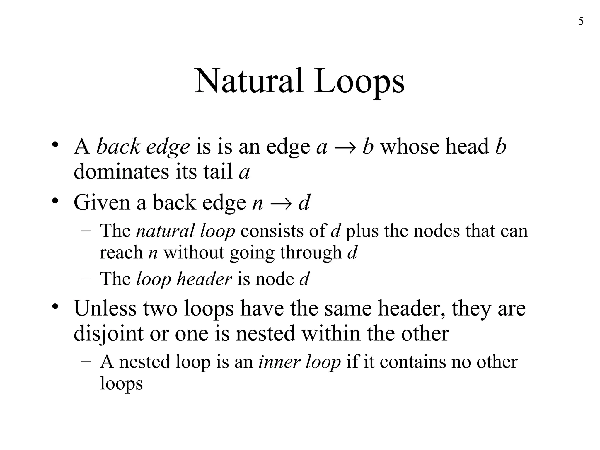
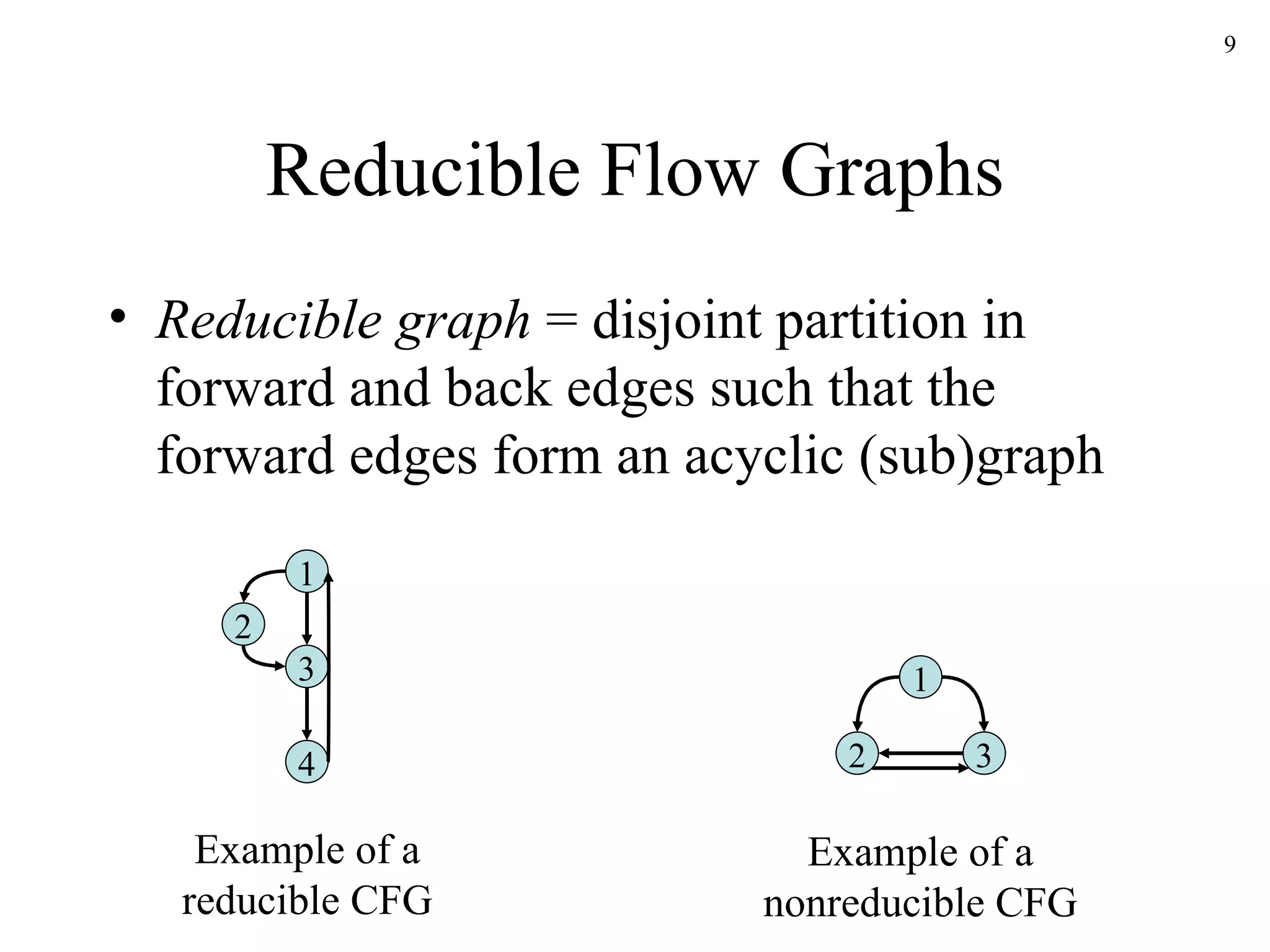
The document discusses code optimization techniques used by compilers, including control flow analysis, data flow analysis, and code transformations. It covers determining loops in a control flow graph using dominators, building dominator trees, and identifying natural loops. It also discusses reaching definitions as a data flow analysis problem and how bit vectors can be used to compute reaching definitions in a conservative manner to ensure safety.

1. Code Optimization Chapter 9 (1 st ed. Ch.10) COP5621 Compiler Construction Copyright Robert van Engelen, Florida State University, 2007-2009

2. The Code Optimizer Control flow analysis: control flow graph Data-flow analysis Transformations Front end Code generator Code optimizer Control- flow analysis Data- flow analysis Transfor- mations

3. Determining Loops in Flow Graphs: Dominators Dominators: d dom n Node d of a CFG dominates node n if every path from the initial node of the CFG to n goes through d The loop entry dominates all nodes in the loop The immediate dominator m of a node n is the last dominator on the path from the initial node to n If d  n and d dom n then d dom m

4. Dominator Trees 1 2 3 4 5 6 7 8 9 10 1 2 3 4 6 5 7 8 9 10 CFG Dominator tree

5. Natural Loops A back edge is is an edge a  b whose head b dominates its tail a Given a back edge n  d The natural loop consists of d plus the nodes that can reach n without going through d The loop header is node d Unless two loops have the same header, they are disjoint or one is nested within the other A nested loop is an inner loop if it contains no other loops

6. Natural Inner Loops Example 1 2 3 4 5 6 7 8 9 10 1 2 3 4 6 5 7 8 9 10 CFG Dominator tree Natural loop for 7 dom 10 Natural loop for 3 dom 4 Natural loop for 4 dom 7

7. Natural Outer Loops Example 1 2 3 4 5 6 7 8 9 10 1 2 3 4 6 5 7 8 9 10 CFG Dominator tree Natural loop for 1 dom 9 Natural loop for 3 dom 8

8. Pre-Headers To facilitate loop transformations, a compiler often adds a preheader to a loop Code motion, strength reduction, and other loop transformations populate the preheader Header Header Preheader

9. Reducible Flow Graphs Reducible graph = disjoint partition in forward and back edges such that the forward edges form an acyclic (sub)graph 1 2 3 4 Example of a reducible CFG 1 2 3 Example of a nonreducible CFG

10. Global Data-Flow Analysis To apply global optimizations on basic blocks, data-flow information is collected by solving systems of data-flow equations Suppose we need to determine the reaching definitions for a sequence of statements S out [ S ] = gen [ S ]  ( in [ S ] - kill [ S ]) d1: i := m-1 d2: j := n d3: j := j-1 B1: B2: B3: out [B1] = gen [B1] = {d1, d2} out [B2] = gen [B2]  {d1} = {d1, d3} d1 reaches B2 and B3 and d2 reaches B2, but not B3 because d2 is killed in B2

11. Reaching Definitions S d : a:=b+c Then, the data-flow equations for S are: gen [ S ] = { d } kill [ S ] = D a - { d } out [ S ] = gen [ S ]  ( in [ S ] - kill [ S ]) where D a = all definitions of a in the region of code is of the form

12. Reaching Definitions S gen [ S ] = gen [ S 2 ]  ( gen [ S 1 ] - kill [ S 2 ]) kill [ S ] = kill [ S 2 ]  ( kill [ S 1 ] - gen [ S 2 ]) in [ S 1 ] = in [ S ] in [ S 2 ] = out [ S 1 ] out [ S ] = out [ S 2 ] is of the form S 2 S 1

13. Reaching Definitions S gen [ S ] = gen [ S 1 ]  gen [ S 2 ] kill [ S ] = kill [ S 1 ]  kill [ S 2 ] in [ S 1 ] = in [ S ] in [ S 2 ] = in [ S ] out [ S ] = out [ S 1 ]  out [ S 2 ] is of the form S 2 S 1

14. Reaching Definitions S gen [ S ] = gen [ S 1 ] kill [ S ] = kill [ S 1 ] in [ S 1 ] = in [ S ]  gen [ S 1 ] out [ S ] = out [ S 1 ] is of the form S 1

15. Example Reaching Definitions d 1 : i := m-1; d 2 : j := n; d 3 : a := u1; do d 4 : i := i+1; d 5 : j := j-1; if e1 then d 6 : a := u2 else d 7 : i := u3 while e2 ; gen ={ d 1 } kill ={ d 4 , d 7 } d 1 gen ={ d 2 } kill ={ d 5 } d 2 gen ={ d 1 , d 2 } kill ={ d 4 , d 5 , d 7 } ; d 3 gen ={ d 3 } kill ={ d 6 } gen ={ d 1 , d 2 , d 3 } kill ={ d 4 , d 5 , d 6 , d 7 } ; gen ={ d 3 , d 4 , d 5 , d 6 , d 7 } kill ={ d 1 , d 2 } do ; gen ={ d 4 } kill ={ d 1 , d 7 } d 4 ; gen ={ d 5 } kill ={ d 2 } d 5 if e1 d 6 d 7 e1 gen ={ d 6 } kill ={ d 3 } gen ={ d 7 } kill ={ d 1 , d 4 } gen ={ d 4 , d 5 } kill ={ d 1 , d 2 , d 7 } gen ={ d 4 , d 5 , d 6 , d 7 } kill ={ d 1 , d 2 } gen ={ d 4 , d 5 , d 6 , d 7 } kill ={ d 1 , d 2 } gen ={ d 6 , d 7 } kill ={}

16. Using Bit-Vectors to Compute Reaching Definitions d 1 : i := m-1; d 2 : j := n; d 3 : a := u1; do d 4 : i := i+1; d 5 : j := j-1; if e1 then d 6 : a := u2 else d 7 : i := u3 while e2 ; d 1 d 2 ; d 3 ; 0011111 1100000 do ; d 4 ; d 5 if e1 d 6 d 7 e1 1110000 0001111 1100000 0001101 1000000 0001001 0100000 0000100 0010000 0000010 0001111 1100000 0001111 1100000 0001100 1100001 0001000 1000001 0000100 0100000 0000010 0010000 0000001 1001000 0000011 0000000

17. Accuracy, Safeness, and Conservative Estimations Conservative : refers to making safe assumptions when insufficient information is available at compile time, i.e. the compiler has to guarantee not to change the meaning of the optimized code Safe : refers to the fact that a superset of reaching definitions is safe (some may have been killed) Accuracy : more and better information enables more code optimizations

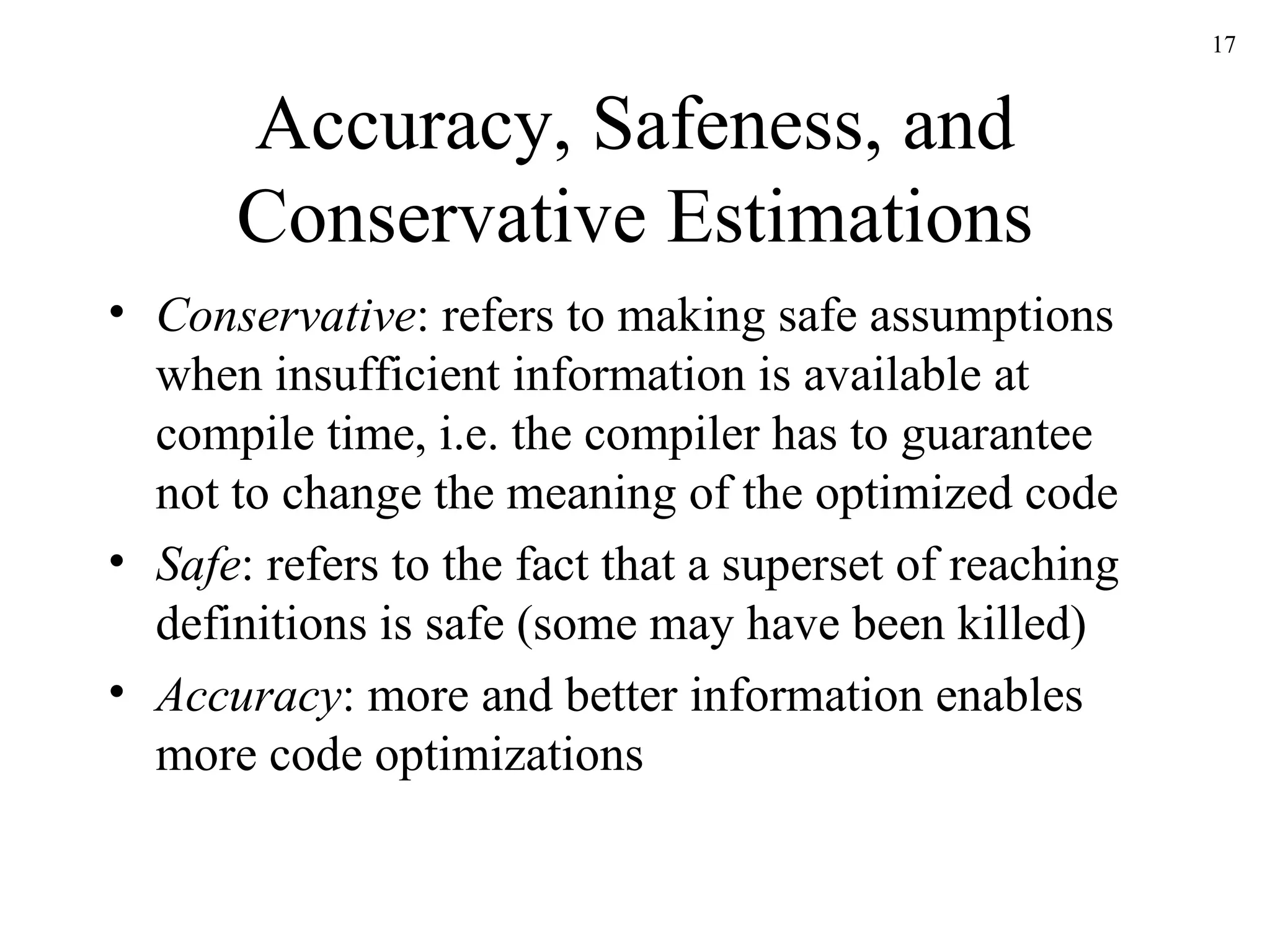
18. Reaching Definitions are a Conservative (Safe) Estimation S 2 S 1 Suppose this branch is never taken Estimation: gen [ S ] = gen [ S 1 ]  gen [ S 2 ] kill [ S ] = kill [ S 1 ]  kill [ S 2 ] Accurate: gen’ [ S ] = gen [ S 1 ] ⊆ gen [ S ] kill’ [ S ] = kill [ S 1 ] ⊇ kill [ S ]

19. Reaching Definitions are a Conservative (Safe) Estimation in [ S 1 ] = in [ S ]  gen [ S 1 ] S 1 Why gen ? S is of the form The problem is that in [ S 1 ] = in [ S ]  out [ S 1 ] makes more sense, but we cannot solve this directly, because out [ S 1 ] depends on in [ S 1 ]

20. Reaching Definitions are a Conservative (Safe) Estimation d : a:=b+c We have: (1) in [ S 1 ] = in [ S ]  out [ S 1 ] (2) out [ S 1 ] = gen [ S 1 ]  ( in [ S 1 ] - kill [ S 1 ]) Solve in [ S 1 ] and out [ S 1 ] by estimating in 1 [ S 1 ] using safe but approximate out [ S 1 ]=  , then re-compute out 1 [ S 1 ] using (2) to estimate in 2 [ S 1 ], etc. in 1 [ S 1 ] = (1) in [ S ]  out [ S 1 ] = in [ S ] out 1 [ S 1 ] = (2) gen [ S 1 ]  ( in 1 [ S 1 ] - kill [ S 1 ]) = gen [ S 1 ]  ( in [ S ] - kill [ S 1 ]) in 2 [ S 1 ] = (1) in [ S ]  out 1 [ S 1 ] = in [ S ]  gen [ S 1 ]  ( in [ S ] - kill [ S 1 ]) = in [ S ]  gen [ S 1 ] out 2 [ S 1 ] = (2) gen [ S 1 ]  ( in 2 [ S 1 ] - kill [ S 1 ]) = gen [ S 1 ]  ( in [ S ]  gen [ S 1 ] - kill [ S 1 ]) = gen [ S 1 ]  ( in [ S ] - kill [ S 1 ]) Because out 1 [ S 1 ] = out 2 [ S 1 ], and therefore in 3 [ S 1 ] = in 2 [ S 1 ], we conclude that in [ S 1 ] = in [ S ]  gen [ S 1 ]