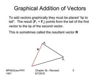
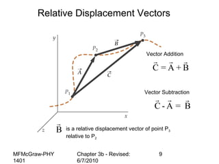
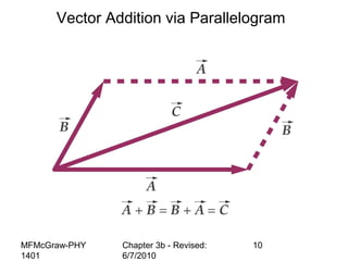
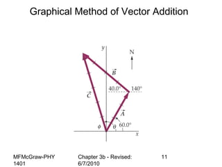
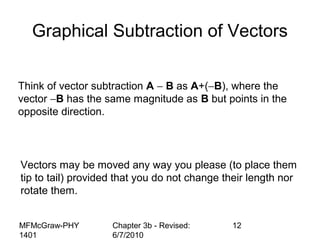
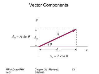
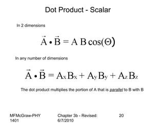
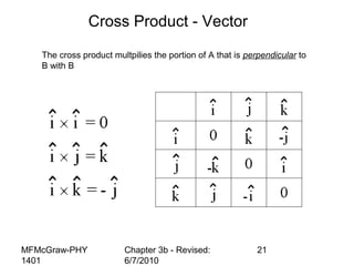
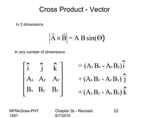
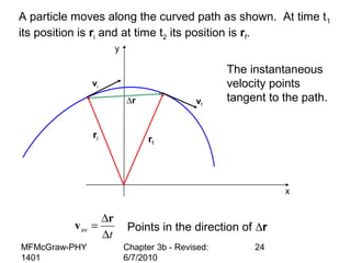
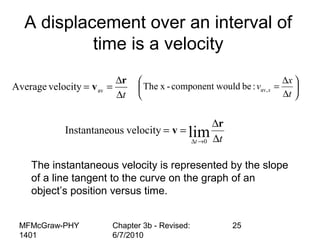
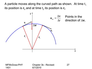
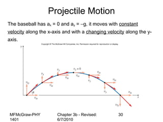
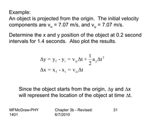
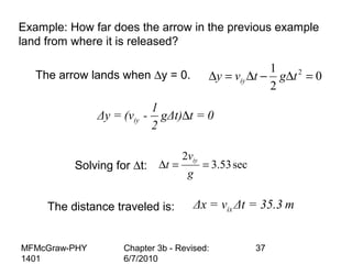
This document summarizes key concepts from a chapter on motion in a plane, including adding and subtracting vectors using graphical and component methods, definitions of velocity and acceleration, and projectile motion where the acceleration along the x-axis is 0 and along the y-axis is -g. Examples of solving projectile motion problems are provided, such as calculating the velocity and position of an object over time or determining where an object lands.

1. MFMcGraw-PHY
1401
Chapter 3b - Revised:
6/7/2010
1
Motion in a Plane
Chapter 3

2. MFMcGraw-PHY
1401
Chapter 3b - Revised:
6/7/2010
2
Motion in a Plane
• Vector Addition
• Velocity
• Acceleration
• Projectile motion

3. MFMcGraw-PHY
1401
Chapter 3b - Revised:
6/7/2010
3
Graphical Addition and Subtraction
of Vectors
A vector is a quantity that has both a
magnitude and a direction. Position is an
example of a vector quantity.
A scalar is a quantity with no direction. The
mass of an object is an example of a scalar
quantity.

4. MFMcGraw-PHY
1401
Chapter 3b - Revised:
6/7/2010
4
Notation
Vector: FF

or
The magnitude of a vector: .oror FF

F
Scalar: m (not bold face; no arrow)
The direction of vector might be “35° south of east”;
“20° above the +x-axis”; or….

5. MFMcGraw-PHY
1401
Chapter 3b - Revised:
6/7/2010
5
To add vectors graphically they must be placed “tip to
tail”. The result (F1 + F2) points from the tail of the first
vector to the tip of the second vector.
This is sometimes called the resultant vector R
F1
F2
R
Graphical Addition of Vectors

6. MFMcGraw-PHY
1401
Chapter 3b - Revised:
6/7/2010
6
Vector Simulation

7. MFMcGraw-PHY
1401
Chapter 3b - Revised:
6/7/2010
7
Examples
• Trig Table
• Vector Components
• Unit Vectors

8. MFMcGraw-PHY
1401
Chapter 3b - Revised:
6/7/2010
8
Types of Vectors

9. MFMcGraw-PHY
1401
Chapter 3b - Revised:
6/7/2010
9
Relative Displacement Vectors
C = A + B
  
C - A = B
  
Vector Addition
Vector Subtraction
B

is a relative displacement vector of point P3
relative to P2

10. MFMcGraw-PHY
1401
Chapter 3b - Revised:
6/7/2010
10
Vector Addition via Parallelogram

11. MFMcGraw-PHY
1401
Chapter 3b - Revised:
6/7/2010
11
Graphical Method of Vector Addition

12. MFMcGraw-PHY
1401
Chapter 3b - Revised:
6/7/2010
12
Think of vector subtraction A − B as A+(−B), where the
vector −B has the same magnitude as B but points in the
opposite direction.
Graphical Subtraction of Vectors
Vectors may be moved any way you please (to place them
tip to tail) provided that you do not change their length nor
rotate them.

13. MFMcGraw-PHY
1401
Chapter 3b - Revised:
6/7/2010
13
Vector Components

14. MFMcGraw-PHY
1401
Chapter 3b - Revised:
6/7/2010
14
Vector Components

15. MFMcGraw-PHY
1401
Chapter 3b - Revised:
6/7/2010
15
Graphical Method of Vector Addition

16. MFMcGraw-PHY
1401
Chapter 3b - Revised:
6/7/2010
16
Unit Vectors in Rectangular Coordinates

17. MFMcGraw-PHY
1401
Chapter 3b - Revised:
6/7/2010
17
Vector Components in Rectangular
Coordinates

18. MFMcGraw-PHY
1401
Chapter 3b - Revised:
6/7/2010
18
x y zA = A i + A j+ A kˆ ˆ ˆ
r
x y zB = B i +B j + B kˆ ˆ ˆ
r
Vectors with Rectangular Unit Vectors

19. MFMcGraw-PHY
1401
Chapter 3b - Revised:
6/7/2010
19
Dot Product - Scalar
The dot product multiplies the portion of A that is parallel to B with B

20. MFMcGraw-PHY
1401
Chapter 3b - Revised:
6/7/2010
20
Dot Product - Scalar
The dot product multiplies the portion of A that is parallel to B with B
In 2 dimensions
In any number of dimensions

21. MFMcGraw-PHY
1401
Chapter 3b - Revised:
6/7/2010
21
Cross Product - Vector
The cross product multpilies the portion of A that is perpendicular to
B with B

22. MFMcGraw-PHY
1401
Chapter 3b - Revised:
6/7/2010
22
x y z
x y z
i j k
A A A
B B B
ˆ ˆ ˆ 
 
 
 
  
y z z y
x z z x
x y x y
= (A B - A B )i
+ (A B - A B ) j
+ (A B - A B ) k
ˆ
ˆ
ˆ
A B = A Bsin( )× Θ
r r
In 2 dimensions
In any number of dimensions
Cross Product - Vector

23. MFMcGraw-PHY
1401
Chapter 3b - Revised:
6/7/2010
23
Velocity

24. MFMcGraw-PHY
1401
Chapter 3b - Revised:
6/7/2010
24
y
x
ri rf
t∆
∆
=
r
vav Points in the direction of ∆r
∆r
vi
The instantaneous
velocity points
tangent to the path.vf
A particle moves along the curved path as shown. At time t1
its position is ri and at time t2 its position is rf.

25. MFMcGraw-PHY
1401
Chapter 3b - Revised:
6/7/2010
25
tt ∆
∆
==
→∆
r
v lim0
velocityousInstantane
The instantaneous velocity is represented by the slope
of a line tangent to the curve on the graph of an
object’s position versus time.
t∆
∆
==
r
vavvelocityAverage 





∆
∆
=
t
x
v x,av:bewouldcomponent-xThe
A displacement over an interval of
time is a velocity

26. MFMcGraw-PHY
1401
Chapter 3b - Revised:
6/7/2010
26
Acceleration

27. MFMcGraw-PHY
1401
Chapter 3b - Revised:
6/7/2010
27
y
x
vi
ri rf
vf
A particle moves along the curved path as shown. At time t1
its position is r0 and at time t2 its position is rf.
∆v
Points in the
direction of ∆v.t∆
∆
=
v
aav

28. MFMcGraw-PHY
1401
Chapter 3b - Revised:
6/7/2010
28
t∆
∆
==
v
aavonacceleratiAverage
A nonzero acceleration changes an
object’s state of motion
Δt 0
Δv
Instantaneous acceleration = a = lim
Δt→
These have interpretations similar to vav and v.

29. MFMcGraw-PHY
1401
Chapter 3b - Revised:
6/7/2010
29
Motion in a Plane with Constant
Acceleration - Projectile
What is the motion of a struck baseball? Once it leaves the
bat (if air resistance is negligible) only the force of gravity
acts on the baseball.
Acceleration due to gravity has a constant value near the
surface of the earth. We call it g = 9.8 m/s2
Only the vertical motion is affected by gravity

30. MFMcGraw-PHY
1401
Chapter 3b - Revised:
6/7/2010
30
The baseball has ax = 0 and ay = −g, it moves with constant
velocity along the x-axis and with a changing velocity along the y-
axis.
Projectile Motion

31. MFMcGraw-PHY
1401
Chapter 3b - Revised:
6/7/2010
31
Example:
An object is projected from the origin. The initial velocity
components are vix = 7.07 m/s, and viy = 7.07 m/s.
Determine the x and y position of the object at 0.2 second
intervals for 1.4 seconds. Also plot the results.
2
f i iy y
f i ix
1
Δy = y - y = v Δt + a Δt
2
Δx = x - x = v Δt
Since the object starts from the origin, ∆y and ∆x
will represent the location of the object at time ∆t.

32. MFMcGraw-PHY
1401
Chapter 3b - Revised:
6/7/2010
32
t (sec) x (meters) y (meters)
0 0 0
0.2 1.41 1.22
0.4 2.83 2.04
0.6 4.24 2.48
0.8 5.66 2.52
1.0 7.07 2.17
1.2 8.48 1.43
1.4 9.89 0.29
Example continued:

33. MFMcGraw-PHY
1401
Chapter 3b - Revised:
6/7/2010
33
0
2
4
6
8
10
12
0 0.5 1 1.5
t (sec)
x,y(m)
This is a plot of the x position (black points) and y position
(red points) of the object as a function of time.
Example continued:

34. MFMcGraw-PHY
1401
Chapter 3b - Revised:
6/7/2010
34
Example continued:
0
0.5
1
1.5
2
2.5
3
0 2 4 6 8 10
x (m)
y(m)
This is a plot of the y position versus x position for the
object (its trajectory). The object’s path is a parabola.

35. MFMcGraw-PHY
1401
Chapter 3b - Revised:
6/7/2010
35
Example (text problem 3.50): An arrow is shot into the air
with θ = 60° and vi = 20.0 m/s.
(a) What are vx and vy of the arrow when t = 3 sec?
The components of the initial
velocity are:
m/s3.17sin
m/s0.10cos
==
==
θ
θ
iiy
iix
vv
vv
At t = 3 sec:
m/s1.12
m/s0.10
−=∆−=∆+=
==∆+=
tgvtavv
vtavv
iyyiyfy
ixxixfx
x
y
60°
vi
CONSTANT

36. MFMcGraw-PHY
1401
Chapter 3b - Revised:
6/7/2010
36
(b) What are the x and y components of the displacement
of the arrow during the 3.0 sec interval?
y
x
r
2
x f i ix x ix
2 2
y f i iy y iy
1
Δr = Δx = x - x = v Δt + a Δt = v Δt +0 = 30.0 m
2
1 1
Δr = Δy = y - y = v Δt + a Δt = v Δt - gΔt = 7.80 m
2 2
Example continued:

37. MFMcGraw-PHY
1401
Chapter 3b - Revised:
6/7/2010
37
Example: How far does the arrow in the previous example
land from where it is released?
The arrow lands when ∆y = 0. 0
2
1 2
=∆−∆=∆ tgtvy iy
Solving for ∆t: sec53.3
2
==∆
g
v
t iy
The distance traveled is: ixΔx = v Δt = 35.3 m
∆iy
1
Δy = (v - gΔt) t = 0
2

38. MFMcGraw-PHY
1401
Chapter 3b - Revised:
6/7/2010
38
Summary
• Adding and subtracting vectors (graphical
method & component method)
• Velocity
• Acceleration
• Projectile motion (here ax = 0 and ay = −g)

39. MFMcGraw-PHY
1401
Chapter 3b - Revised:
6/7/2010
39
Projectiles Examples
• Problem solving strategy
• Symmetry of the motion
• Dropped from a plane
• The home run