Amazon.comThe three main activities that e.docx

Amazon.com
The three main activities that exist within Amazon’s logistics
sector are listed below:
Order Processing
Inventory Management
Freight Transportation
Logistics (IT)Management System
Bowersox, D. J., Closs, D. J., & Cooper, M. B. (2002). Supply
chain logistics management (Vol. 2). New York, NY: McGraw-
Hill
2
The fourth functional area of Amazon logistics place take
within.
Warehousing, Material Handling and Packaging
Facility Networks

Logistics (IT) Management System cont.
Hill
3
Amazon Web Services
Amazon Simple Storage Service
Information System
Customer Relationship Management
Amazon IT Management Systems
Chaffey, D. et al (2004) Business Information Management:
Improving Performance using Information Systems (1st Edition)
Prentice Hall Pearson Education. England

4
Rail
Truck
Air
Intermodal Transportation
Cost of transport
Total system cost
Speed of transportation
Outsourcing
Third-party logistics service provider (3PL)
Transportation
Hill.
5
Distribution Management Operations
Yet Another Massive Market on the ... - media.cygnus.com.
(n.d.). Retrieved April 5, 2016, from
http://media.cygnus.com/files/base/FL/document/2015/10/RW_
Baird_AMZN2015-10-19_report.pdf
6

Hill.
Chaffey, D. et al (2004) Business Information Management:
Improving Performance using Information Systems (1st Edition)
Prentice Hall Pearson Education. England
Stock, J. R., & Lambert, D. M. (2001). Strategic logistics
management (Vol. 4). Boston, MA: McGraw-Hill/Irwin.
Kerzner, H. R. (2013). Project management: a systems approach
to planning, scheduling, and controlling. John Wiley & Sons.
Hill, Charles W.L., Schilling, Melissa A., & Jones, Gareth R.
(2016). Strategic Management: Theory & Cases: an Integrated
Approach. South-Western Pub.
References
398
Chapter Preview Now that we have some basic techniques for
evaluating integrals,
we turn our attention to the uses of integration, which are
virtually endless. We first illus-
trate the general rule that if the rate of change of a quantity is
known, then integration
can be used to determine the net change or the future value of
that quantity over a certain
time interval. Next, we explore some rich geometric
applications of integration: comput-

ing the area of regions bounded by several curves, the volume
and surface area of three-
dimensional solids, and the length of curves. A variety of
physical applications of integration
include finding the work done by a variable force and
computing the total force exerted
by water behind a dam. All of these applications are unified by
their use of the slice-and-
sum strategy. We end this chapter by revisiting the logarithmic
function, exploring the many
applications of the exponential function, and introducing
hyperbolic functions.
6.1 Velocity and Net Change
In previous chapters, we established the relationship between
the position and velocity
of an object moving along a line. With integration, we can now
say much more about
this relationship. Once we relate velocity and position through
integration, we can make
analogous observations about a variety of other practical
problems, which include fluid
flow, population growth, manufacturing costs, and production
and consumption of natu-
ral resources. The ideas in this section come directly from the
Fundamental Theorem of
Calculus, and they are among the most powerful applications of
calculus.
Velocity, Position, and Displacement
Suppose you are driving along a straight highway and your
position relative to a reference
point or origin is s1t2 for times t Ú 0. Your displacement over a
time interval 3a, b4 is the
change in the position s1b2 - s1a2 (Figure 6.1). If s1b2 7 s1a2,
then your displacement

is positive; when s1b2 6 s1a2, your displacement is negative.
6.1 Velocity and Net Change
6.2 Regions Between Curves
6.3 Volume by Slicing
6.4 Volume by Shells
6.5 Length of Curves
6.6 Surface Area
6.7 Physical Applications
6.8 Logarithmic and Exponential
Functions Revisited
6.9 Exponential Models
6.10 Hyperbolic Functions
Applications of Integration
6
s(b)s ! 0 s(a) s (line of motion)
Position at t ! a Position at t ! b " a
Displacement ! s (b) # s (a) " 0
s(a)s ! 0 s(b) s (line of motion)
Position at t ! b " a Position at t ! a

Displacement ! s (b) # s (a) $ 0Figure 6.1
M06_BRIG7345_02_SE_C06.1.indd 398 21/10/13 9:20 PM
6.1 Velocity and Net Change 399
Now assume that v1t2 is the velocity of the object at a
particular time t. Recall from
Chapter 3 that v1t2 = s′1t2, which means that s is an
antiderivative of v. From the Funda-
mental Theorem of Calculus, it follows that
L
b
a
v1t2 dt = Lba s′1t2 dt = s1b2 - s1a2 = displacement.
We see that the definite integral 1ba v1t2 dt is the displacement
(change in position) be-
tween times t = a and t = b. Equivalently, the displacement over
the time interval 3a, b4
is the net area under the velocity curve over 3a, b4 (Figure
6.2a).
Not to be confused with the displacement is the distance
traveled over a time interval,
which is the total distance traveled by the object, independent
of the direction of motion.
If the velocity is positive, the object moves in the positive
direction and the displacement
equals the distance traveled. However, if the velocity changes
sign, then the displacement

and the distance traveled are not generally equal.
QUICK CHECK 1 A police officer leaves his station on a north-
south freeway at 9 a.m., trav-
eling north (the positive direction) for 40 mi between 9 a.m. and
10 a.m. From 10 a.m. to
11 a.m., he travels south to a point 20 mi south of the station.
What are the distance trav-
eled and the displacement between 9 a.m. and 11 a.m.?
To compute the distance traveled, we need the magnitude, but
not the sign, of the
velocity. The magnitude of the velocity " v1t2 " is called the
speed. The distance traveled over
a small time interval dt is " v1t2 " dt (speed multiplied by
elapsed time). Summing these dis-
tances, the distance traveled over the time interval 3a, b4 is the
integral of the speed; that is,
distance traveled = L
b
a
" v1t2 " dt.
As shown in Figure 6.2b, integrating the speed produces the
area (not net area)
bounded by the velocity curve and the t-axis, which corresponds
to the distance traveled.
The distance traveled is always nonnegative.Figure 6.2
y
t
t

a b
a
b
y
O
O
y ! v(t)
Area ! A1
Area ! A1
Area ! A2
Area ! A2
Displacement ! A1 " A2 ! ! v(t) dt
a
b
Distance traveled ! A1 # A2 ! ! "v(t)" dt
a
b
y ! "v(t)"
(a)

(b)
DEFINITION Position, Velocity, Displacement, and Distance
1. The position of an object moving along a line at time t,
denoted s1t2, is the loca-
tion of the object relative to the origin.
2. The velocity of an object at time t is v1t2 = s′1t2.
3. The displacement of the object between t = a and t = b 7 a is
s1b2 - s1a2 = Lba v1t2 dt.
4. The distance traveled by the object between t = a and t = b 7
a is
L
b
a
" v1t2 " dt,
where " v1t2 " is the speed of the object at time t.
QUICK CHECK 2 Describe a possible motion of an object along
a line for 0 … t … 5 for
which the displacement and the distance traveled are different.
M06_BRIG7345_02_SE_C06.1.indd 399 21/10/13 11:29 AM
400 Chapter 6 Applications of Integration
EXAMPLE 1 Displacement from velocity A jogger runs along a
straight road with
velocity (in mi/hr) v1t2 = 2t2 - 8t + 6, for 0 … t … 3, where t

is measured in hours.
a. Graph the velocity function over the interval 30, 34.
Determine when the jogger moves
in the positive direction and when she moves in the negative
direction.
b. Find the displacement of the jogger (in miles) on the time
intervals 30, 14, 31, 34, and 30, 34. Interpret these results.
c. Find the distance traveled over the interval 30, 34.
SOLUTION
a. By solving v1t2 = 2t2 - 8t + 6 = 21t - 121t - 32 = 0, we find
that the velocity
is zero at t = 1 and t = 3; these values are the t-intercepts of the
graph of v, which is
an upward-opening parabola with a v-intercept of 6 (Figure
6.3a). The velocity is posi-
tive on the interval 0 … t 6 1, which means the jogger moves in
the positive s direc-
tion. For 1 6 t 6 3, the velocity is negative and the jogger moves
in the negative s
direction.
b. The displacement (in miles) over the interval 30, 14 is
s112 - s102 = L10 v1t2 dt
= L
1
0
12t2 - 8t + 62 dt Substitute for v.
= a2
3

t3 - 4t2 + 6tb ` 1
0
=
8
3
. Evaluate integral.
A similar calculation shows that the displacement over the
interval 31, 34 is
s132 - s112 = L31 v1t2 dt = - 83.
Over the interval 30, 34, the displacement is 83 + 1-832 = 0,
which means the jogger
returns to the starting point after three hours.
c. From part (b), we can deduce the total distance traveled by
the jogger. On the interval 30, 14, the distance traveled is 83
mi; on the interval 31, 34, the distance traveled is also
8
3 mi. Therefore, the distance traveled on 30, 34 is 163 mi.
Alternatively (Figure 6.3b),
we can integrate the speed and get the same result:
L
3
0
! v1t2 ! dt = L10 12t2 - 8t + 62 dt + L31 1-12t2 - 8t + 622 dt
Definition of ! v1t2 !
= a 2
3
t3 - 4t2 + 6tb ` 1

0
+ a - 2
3
t3 + 4t2 - 6tb ` 3
1
Evaluate integrals.
=
16
3
. Simplify.
Related Exercises 7–14
Figure 6.3
6
4
2
!2
310
v
t
6

4
2
!2
321
!v!
t0
0
1
1
3
0
3
v (t) " 2t2 ! 8t # 6 !v (t)! " !2t2 ! 8t # 6!
Displacement
" " v(t) dt "
Displacement
" " v(t) dt "
Distance traveled from t " 0 to t " 3
is " !v (t)! dt " Displacement from t " 0to t " 3 is " 0.

Area "
Area "
Area "
Area "
(a) (b)
6
4
2
!2
310
v
t
6
4
2
!2
321
!v!

t0
0
1
1
3
0
3
v (t) " 2t2 ! 8t # 6 !v (t)! " !2t2 ! 8t # 6!
Displacement
" " v(t) dt "
Displacement
" " v(t) dt "
Distance traveled from t " 0 to t " 3
is " !v (t)! dt " Displacement from t " 0to t " 3 is " 0.
Area "
Area "
Area "
Area "
(a) (b)

M06_BRIG7345_02_SE_C06.1.indd 400 21/10/13 11:29 AM
Future Value of the Position Function
To find the displacement of an object, we do not need to know
its initial position. For ex-
ample, whether an object moves from s = -20 to s = -10 or from
s = 50 to s = 60,
its displacement is 10 units. What happens if we are interested
in the actual position of the
object at some future time?
Suppose we know the velocity of an object and its initial
position s102. The goal is to
find the position s1t2 at some future time t Ú 0. The
Fundamental Theorem of Calculus
gives us the answer directly. Because the position s is an
antiderivative of the velocity v,
we have
L
t
0
v1x2 dx = L t0 s′1x2 dx = s1x2 ` t0 = s1t2 - s102.
Rearranging this expression leads to the following result.
➤ Note that t is the independent variable of
the position function. Therefore, another
(dummy) variable, in this case x, must be
used as the variable of integration.

➤ Theorem 6.1 is a consequence (actually a
statement) of the Fundamental Theorem
of Calculus.
THEOREM 6.1 Position from Velocity
Given the velocity v1t2 of an object moving along a line and its
initial position
s102, the position function of the object for future times t Ú 0 is
s1t2 = s102 + L t0 v1x2 dx.
position initial
displacement
at t position
over 30, t4dee
Theorem 6.1 says that to find the position s1t2, we add the
displacement over the interval 30, t4 to the initial position s102.
QUICK CHECK 3 Is the position s1t2 a number or a function?
For fixed times t = a and
t = b, is the displacement s1b2 - s1a2 a number or a function?
There are two equivalent ways to determine the position
function:
Using antiderivatives (Section 4.9)
Using Theorem 6.1
The latter method is usually more efficient, but either method
produces the same result.
The following example illustrates both approaches.

EXAMPLE 2 Position from velocity A block hangs at rest from
a massless spring at
the origin 1s = 02. At t = 0, the block is pulled downward 14 m
to its initial position
s102 = -14 and released (Figure 6.4). Its velocity 1in m>s2 is
given by v1t2 = 14 sin t, for
t Ú 0. Assume that the upward direction is positive.
a. Find the position of the block, for t Ú 0.
b. Graph the position function, for 0 … t … 3p.
c. When does the block move through the origin for the first
time?
d. When does the block reach its highest point for the first time
and what is its position at
that time? When does the block return to its lowest point?Figure
6.4
s(0) ! "E
Position of
the block
at time t ! 0
Position of
the block
at a later time t
0
0.25
0.50
0.75
1.00

"0.25
s(t)
s
0
0.25
0.50
0.75
1.00
"0.25
s
M06_BRIG7345_02_SE_C06.1.indd 401 21/10/13 11:29 AM
SOLUTION As shown in Figure 6.9, the growth rate is large
when t is small (plenty of food
and space) and decreases as t increases. Knowing that the initial
population is N102 =
100 cells, we can find the population N1t2 at any future time t
Ú 0 using Theorem 6.3:
N1t2 = N102 + L t0 N′1x2 dx
= 100 + L

t
0
90e-0.1x dx
()* c
N102 N′1x2
= 100 + c a 90-0.1 be-0.1x d ` t0 Fundamental Theorem
= 1000 - 900e-0.1t. Simplify.
The graph of the population function (Figure 6.10) shows that
the population increases,
but at a decreasing rate. Note that the initial condition N102 =
100 cells is satisfied and
that the population size approaches 1000 cells as t S ∞ .
Figure 6.9
t2010
N !
90
60
30
The growth rate is initially
90 cells/hr and decreases as
time increases.
N !(t) " 90e#0.1t
Time (hr)

G
ro
w
th
ra
te
(c
el
ls
/h
r)
0
0 t30252015105
N
1000
800
600
400
200
Time (hr)

C
el
l p
op
ul
at
io
n
Max. population ! 1000
N(t) ! 1000 " 900e"0.1t
N(10) " N(5) ! 215 cells
N(15) " N(10) ! 130 cells
The population is growing
at a decreasing rate.
Figure 6.10
EXAMPLE 6 Production costs A book publisher estimates that
the marginal cost of a
particular title (in dollars/book) is given by
C′1x2 = 12 - 0.0002x,
where 0 … x … 50,000 is the number of books printed. What is
the cost of producing the
12,001st through the 15,000th book?
SOLUTION Recall from Section 3.6 that the cost function C1x2
is the cost required to
produce x units of a product. The marginal cost C′1x2 is the

approximate cost of produc-
ing one additional unit after x units have already been produced.
The cost of producing
books x = 12,001 through x = 15,000 is the cost of producing
15,000 books minus
the cost of producing the first 12,000 books. Therefore, the cost
in dollars of producing
books 12,001 through 15,000 is
C115,0002 - C112,0002 = L15,00012,000 C′1x2 dx
= L
15,000
12,000
112 - 0.0002x2 dx Substitute for C′1x2.
= 112x - 0.0001x22 ` 15,000
12,000
Fundamental Theorem
= 27,900. Simplify.
➤ Although x is a positive integer (the
number of books produced), we treat it as
a continuous variable in this example.
QUICK CHECK 6 Is the cost of increas-
ing the production from 9000 books
to 12,000 books in Example 6 more
or less than the cost of increasing
the production from 12,000 books to
15,000 books? Explain.

M06_BRIG7345_02_SE_C06.1.indd 406 21/10/13 11:30 AM
SECTION 6.1 EXERCISES
Review Questions
1. Explain the meaning of position, displacement, and distance
traveled as they apply to an object moving along a line.
2. Suppose the velocity of an object moving along a line is
positive.
Are displacement and distance traveled equal? Explain.
3. Given the velocity function v of an object moving along a
line,
explain how definite integrals can be used to find the displace-
ment of the object.
4. Explain how to use definite integrals to find the net change in
a
quantity, given the rate of change of that quantity.
5. Given the rate of change of a quantity Q and its initial value
Q102,
explain how to find the value of Q at a future time t Ú 0.
6. What is the result of integrating a population growth rate
between
times t = a and t = b, where b 7 a?
Basic Skills
7. Displacement and distance from velocity Consider the graph

shown in the figure, which gives the velocity of an object mov-
ing along a line. Assume time is measured in hours and distance
is measured in miles. The areas of three regions bounded by the
velocity curve and the t-axis are also given.
t
v
543210
12
16
10
a. On what intervals is the object moving in the positive
direction?
b. What is the displacement of the object over the interval 30,
34?
c. What is the total distance traveled by the object over the
interval 31, 54?
d. What is the displacement of the object over the interval 30,
54?
e. Describe the position of the object relative to its initial
position
after 5 hours.
8. Displacement and distance from velocity Consider the
velocity
function shown below of an object moving along a line. Assume
time is measured in seconds and distance is measured in meters.
The areas of four regions bounded by the velocity curve and the

t-axis are also given.
t
v
876543210
10
6
20
14
a. On what intervals is the object moving in the negative
direction?
b. What is the displacement of the object over the interval 32,
64?
c. How far does the object travel over the interval 30, 64?
d. What is the displacement of the object over the interval 30,
84?
e. Describe the position of the object relative to its initial
position
after 8 hours.
9–14. Displacement from velocity Assume t is time measured in
sec-
onds and velocities have units of m>s.
a. Graph the velocity function over the given interval. Then
determine
when the motion is in the positive direction and when it is in
the

negative direction.
b. Find the displacement over the given interval.
c. Find the distance traveled over the given interval.
9. v1t2 = 6 - 2t on 0 … t … 6
10. v1t2 = 10 sin 2t on 0 … t … 2p
11. v1t2 = t2 - 6t + 8 on 0 … t … 5
12. v1t2 = - t2 + 5t - 4 on 0 … t … 5
13. v1t2 = t3 - 5t2 + 6t on 0 … t … 5
14. v1t2 = 50e-2t on 0 … t … 4
15–20. Position from velocity Consider an object moving along
a line
with the following velocities and initial positions.
a. Graph the velocity function on the given interval and
determine
when the object is moving in the positive direction and when it
is
moving in the negative direction.
b. Determine the position function, for t Ú 0, using both the
antiderivative method and the Fundamental Theorem of
Calculus
(Theorem 6.1). Check for agreement between the two methods.
c. Graph the position function on the given interval.
15. v1t2 = sin t on 30, 2p4; s102 = 1
16. v1t2 = - t3 + 3t2 - 2t on 30, 34; s102 = 4
17. v1t2 = 6 - 2t on 30, 54; s102 = 0
18. v1t2 = 3 sin pt on 30, 44; s102 = 1
19. v1t2 = 9 - t2 on 30, 44; s102 = -2
20. v1t2 = 1>1t + 12 on 30, 84; s102 = -4
21. Oscillating motion A mass hanging from a spring is set in

motion, and its ensuing velocity is given by v1t2 = 2p cos pt,
for t Ú 0. Assume that the positive direction is upward and that
s102 = 0.
a. Determine the position function, for t Ú 0.
b. Graph the position function on the interval 30, 44.
c. At what times does the mass reach its low point the first three
times?
d. At what times does the mass reach its high point the first
three
times?
22. Cycling distance A cyclist rides down a long straight road at
a
velocity (in m>min) given by v1t2 = 400 - 20t, for 0 … t … 10,
where t is measured in minutes.
a. How far does the cyclist travel in the first 5 min?
b. How far does the cyclist travel in the first 10 min?
c. How far has the cyclist traveled when her velocity is
250 m>min?
T
T
T
M06_BRIG7345_02_SE_C06.1.indd 407 21/10/13 3:11 PM

23. Flying into a headwind The velocity (in mi>hr) of an
airplane
flying into a headwind is given by v1t2 = 30116 - t22, for
0 … t … 3. Assume that s102 = 0 and t is measured in hours.
a. Determine and graph the position function, for 0 … t … 3.
b. How far does the airplane travel in the first 2 hr?
c. How far has the airplane traveled at the instant its velocity
reaches 400 mi>hr?
24. Day hike The velocity (in mi>hr) of a hiker walking along a
straight trail is given by v1t2 = 3 sin2 1pt>22, for 0 … t … 4.
Assume that s102 = 0 and t is measured in hours.
a. Determine and graph the position function, for 0 … t … 4.
1Hint: sin2 t = 1211 - cos 2t2.2
b. What is the distance traveled by the hiker in the first 15 min
of
the hike?
c. What is the hiker’s position at t = 3?
25. Piecewise velocity The velocity of a (fast) automobile on a
straight highway is given by the function
v1t2 = c 3t if 0 … t 6 2060 if 20 … t 6 45
240 - 4t if t Ú 45,
where t is measured in seconds and v has units of m>s.
a. Graph the velocity function, for 0 … t … 70. When is the
velocity a maximum? When is the velocity zero?
b. What is the distance traveled by the automobile in the first 30
s?
c. What is the distance traveled by the automobile in the first 60
s?
d. What is the position of the automobile when t = 75?

26. Probe speed A data collection probe is dropped from a
stationary
balloon, and it falls with a velocity (in m>s) given by v1t2 =
9.8t,
neglecting air resistance. After 10 s, a chute deploys and the
probe
immediately slows to a constant speed of 10 m>s, which it
main-
tains until it enters the ocean.
a. Graph the velocity function.
b. How far does the probe fall in the first 30 s after it is
released?
c. If the probe was released from an altitude of 3 km, when does
it enter the ocean?
27–34. Position and velocity from acceleration Find the position
and
velocity of an object moving along a straight line with the given
accel-
eration, initial velocity, and initial position.
27. a1t2 = -32, v102 = 70, s102 = 10
28. a1t2 = -32, v102 = 50, s102 = 0
29. a1t2 = -9.8, v102 = 20, s102 = 0
30. a1t2 = e-t, v102 = 60, s102 = 40
31. a1t2 = -0.01t, v102 = 10, s102 = 0
32. a1t2 = 201t + 222, v102 = 20, s102 = 10
33. a1t2 = cos 2t, v102 = 5, s102 = 7
34. a1t2 = 2t1t2 + 122, v102 = 0, s102 = 0
35. Acceleration A drag racer accelerates at a1t2 = 88 ft>s2.
Assume
that v102 = 0, s102 = 0, and t is measured in seconds.

a. Determine and graph the position function, for t Ú 0.
b. How far does the racer travel in the first 4 seconds?
c. At this rate, how long will it take the racer to travel 14 mi?
d. How long does it take the racer to travel 300 ft?
e. How far has the racer traveled when it reaches a speed of
178 ft>s?
36. Deceleration A car slows down with an acceleration of
a1t2 = -15 ft>s2. Assume that v102 = 60 ft>s, s102 = 0, and t
is measured in seconds.
a. Determine and graph the position function, for t Ú 0.
b. How far does the car travel in the time it takes to come to
rest?
37. Approaching a station At t = 0, a train approaching a station
begins decelerating from a speed of 80 mi>hr according to the
acceleration function a1t2 = -128011 + 8t2-3, where t Ú 0 is
measured in hours. How far does the train travel between t = 0
and t = 0.2? Between t = 0.2 and t = 0.4? The units of accel-
eration are mi>hr2.
38. Peak oil extraction The owners of an oil reserve begin
extract-
ing oil at time t = 0. Based on estimates of the reserves, suppose
the projected extraction rate is given by Q′1t2 = 3t2 140 - t22,
where 0 … t … 40, Q is measured in millions of barrels, and t is
measured in years.
a. When does the peak extraction rate occur?
b. How much oil is extracted in the first 10, 20, and 30 years?
c. What is the total amount of oil extracted in 40 years?
d. Is one-fourth of the total oil extracted in the first one-fourth
of

the extraction period? Explain.
39. Oil production An oil refinery produces oil at a variable rate
given by
Q′1t2 = c 800 if 0 … t 6 302600 - 60t if 30 … t 6 40
200 if t Ú 40,
where t is measured in days and Q is measured in barrels.
a. How many barrels are produced in the first 35 days?
b. How many barrels are produced in the first 50 days?
c. Without using integration, determine the number of barrels
produced over the interval 360, 804.
40–43. Population growth
40. Starting with an initial value of P102 = 55, the population of
a prairie dog community grows at a rate of P′1t2 = 20 - t>5
(prairie dogs>month), for 0 … t … 200, where t is measured in
months.
a. What is the population 6 months later?
b. Find the population P1t2, for 0 … t … 200.
41. When records were first kept 1t = 02, the population of a
rural town
was 250 people. During the following years, the population
grew at
a rate of P′1t2 = 3011 + 1t2, where t is measured in years.
a. What is the population after 20 years?
b. Find the population P1t2 at any time t Ú 0.
42. The population of a community of foxes is observed to
fluctuate on

a 10-year cycle due to variations in the availability of prey.
When
population measurements began 1t = 02, the population was 35
foxes. The growth rate in units of foxes>year was observed to
be
P′1t2 = 5 + 10 sin pt
5
.
a. What is the population 15 years later? 35 years later?
b. Find the population P1t2 at any time t Ú 0.
M06_BRIG7345_02_SE_C06.1.indd 408 21/10/13 11:30 AM
43. A culture of bacteria in a Petri dish has an initial popula-
tion of 1500 cells and grows at a rate 1in cells>day2 of
N′1t2 = 100e-0.25t. Assume t is measured in days.
a. What is the population after 20 days? After 40 days?
b. Find the population N1t2 at any time t Ú 0.
44. Flow rates in the Spokane River The daily discharge of the
Spo-
kane River as it flows through Spokane, Washington, in April
and
June is modeled by the functions
r11t2 = 0.25t2 + 37.46t + 722.47 1April2 and
r21t2 = 0.90t2 - 69.06t + 2053.12 1June2,
where the discharge is measured in millions of cubic feet per

day
and t = 1 corresponds to the first day of the month (see figure).
t
r
0
15 25205 100
500
1000
1500
2000
r2(t) ! 0.90t
2 " 69.06t # 2053.12
r1(t) ! 0.25t
2 # 37.46t # 722.47
a. Determine the total amount of water that flows through
Spokane in April (30 days).
b. Determine the total amount of water that flows through
Spokane in June (30 days).
c. The Spokane River flows out of Lake Coeur d’Alene, which
contains approximately 0.67 mi3 of water. Determine the per-
centage of Lake Coeur d’Alene’s volume that flows through
Spokane in April and June.
45–48. Marginal cost Consider the following marginal cost

functions.
a. Find the additional cost incurred in dollars when production
is
increased from 100 units to 150 units.
b. Find the additional cost incurred in dollars when production
is
increased from 500 units to 550 units.
45. C′1x2 = 2000 - 0.5x 46. C′1x2 = 200 - 0.05x
47. C′1x2 = 300 + 10x - 0.01x2
48. C′1x2 = 3000 - x - 0.001x2
Further Explorations
49. Explain why or why not Determine whether the following
statements are true and give an explanation or counterexample.
a. The distance traveled by an object moving along a line is the
same as the displacement of the object.
b. When the velocity is positive on an interval, the displacement
and the distance traveled on that interval are equal.
c. Consider a tank that is filled and drained at a flow rate
of V′1t2 = 1 - t2>100 1gal>min2, for t Ú 0, where t is
measured in minutes. It follows that the volume of water in the
tank increases for 10 min and then decreases until the tank is
empty.
d. A particular marginal cost function has the property that it is
positive and decreasing. The cost of increasing production
from A units to 2A units is greater than the cost of increasing
production from 2A units to 3A units.
50–51. Velocity graphs The figures show velocity functions for

motion
along a straight line. Assume the motion begins with an initial
position
of s102 = 0. Determine the following:
a. The displacement between t = 0 and t = 5
b. The distance traveled between t = 0 and t = 5
c. The position at t = 5
d. A piecewise function for s1t2
50.
t51
3
1
v
0
51.
t51
3
1
v
0
52–55. Equivalent constant velocity Consider the following
veloc-
ity functions. In each case, complete the sentence: The same
distance

could have been traveled over the given time period at a
constant
velocity of ________.
52. v1t2 = 2t + 6, for 0 … t … 8
53. v1t2 = 1 - t2>16, for 0 … t … 4
54. v1t2 = 2 sin t, for 0 … t … p
55. v1t2 = t125 - t221>2, for 0 … t … 5
56. Where do they meet? Kelly started at noon 1t = 02 riding a
bike from Niwot to Berthoud, a distance of 20 km, with veloc-
ity v1t2 = 15>1t + 122 (decreasing because of fatigue). Sandy
started at noon 1t = 02 riding a bike in the opposite direction
from Berthoud to Niwot with velocity u1t2 = 20>1t + 122 (also
decreasing because of fatigue). Assume distance is measured in
kilometers and time is measured in hours.
a. Make a graph of Kelly’s distance from Niwot as a function of
time.
b. Make a graph of Sandy’s distance from Berthoud as a
function
of time.
c. When do they meet? How far has each person traveled when
they meet?
d. More generally, if the riders’ speeds are v1t2 = A>1t + 122
and u1t2 = B>1t + 122 and the distance between the towns is
D, what conditions on A, B, and D must be met to ensure that
the riders will pass each other?
e. Looking ahead: With the velocity functions given in part (d),
make a conjecture about the maximum distance each person
can ride (given unlimited time).

57. Bike race Theo and Sasha start at the same place on a
straight
road, riding bikes with the following velocities (measured in
mi>hr). Assume t is measured in hours.
Theo: vT1t2 = 10, for t Ú 0
Sasha: vS1t2 = 15t, for 0 … t … 1 and vS1t2 = 15, for t 7 1
a. Graph the velocity functions for both riders.
b. If the riders ride for 1 hr, who rides farther? Interpret your
answer geometrically using the graphs of part (a).
c. If the riders ride for 2 hr, who rides farther? Interpret your
answer geometrically using the graphs of part (a).
M06_BRIG7345_02_SE_C06.1.indd 409 21/10/13 11:30 AM
In cases such as these, we treat y as the independent variable
and divide the
interval 3c, d4 into n subintervals of width ∆y = 1d - c2>n
(Figure 6.17). On the
kth subinterval, a point yk
* is selected, and we construct a rectangle that extends
from the left curve to the right curve. The kth rectangle has
length f 1yk*2 - g1yk*2,
so the area of the kth rectangle is 1 f 1yk*2 - g1yk*22∆y. The
area of the region is
approximated by the sum of the areas of the rectangles. In the
limit as n S ∞ and
∆y S 0, the area of the region is given as the definite integral

A = lim
nS∞
a
n
k = 1
1 f 1yk*2 - g1yk*22∆y = Ldc 1 f 1y2 - g1y22 dy.
➤ This area formula is analogous to the one
given on page 412; it is now expressed
with respect to the y-axis. In this case,
f 1y2 - g1y2 is the length of a rectangle
and dy represents its width. We sum
(integrate) the areas of the rectangles 1 f 1y2 - g1y22 dy to
obtain the area of
the region.
Given these points of intersection, we see that the region R1 is
bounded by
y = -x2 + 3x + 6 and y = -2x on the interval 3-1, 04. Similarly,
region R2 is
bounded by y = -x2 + 3x + 6 and y = 2x on 30, 34 (Figure
6.15b). Therefore,
A = L
0
-1
11-x2 + 3x + 62 - 1-2x2 2 dx + L30 11-x2 + 3x + 62 - 2x2 dx
(1++++++)++++++* (++++++)+++++1*
area of region R1 area of region R2
= L

0
-1
1-x2 + 5x + 62 dx + L30 1-x2 + x + 62 dx Simplify.
= a - x3
3
+ 5
2
x2 + 6xb ` 0
-1
+ a - x3
3
+ 1
2
x2 + 6xb ` 3
0
Fundamental Theorem
= 0 - a 1
3
+ 5
2
- 6b + a -9 + 9
2
+ 18b - 0 = 50
3

. Simplify.
Integrating with Respect to y
There are occasions when it is convenient to reverse the roles of
x and y. Consider the
regions shown in Figure 6.16 that are bounded by the graphs of
x = f 1y2 and x = g1y2,
where f 1y2 Ú g1y2, for c … y … d (which implies that the
graph of f lies to the right
of the graph of g). The lower and upper boundaries of the
regions are y = c and y = d,
respectively.
Figure 6.16
x x
x
d
c
O
y
d
c
O
y

d
c
O
y
x ! g(y) x ! g(y)
x ! g(y)
x ! f (y) x ! f (y)
x ! f (y)
x
d
c
!y
f (yk*) " g(yk*)
x # g(y) x # f (y)
O
Area of region: A !
k#1
n
$ ( f (yk*) " g(yk*)) !y

( f (yk*), yk*)
(g(yk*), yk*)
y
Area of kth rectangle
# ( f (yk*) " g(yk*)) !y
yk*
Figure 6.17
DEFINITION Area of a Region Between Two Curves with
Respect to y
Suppose that f and g are continuous functions with f 1y2 Ú
g1y2 on the interval 3c, d4.
The area of the region bounded by the graphs x = f 1y2 and x =
g1y2 on 3c, d4 is
A = L
d
c
1 f 1y2 - g1y22 dy.
M06_BRIG7345_02_SE_C06.2.indd 414 21/10/13 11:32 AM
6.2 Regions Between Curves 415
EXAMPLE 3 Integrating with respect to y Find the area of the
region R bounded by
the graphs of y = x3, y = x + 6, and the x-axis.

SOLUTION The area of this region could be found by
integrating with respect to x. But
this approach requires splitting the region into two pieces
(Figure 6.18). Alternatively,
we can view y as the independent variable, express the
bounding curves as functions of y,
and make horizontal slices parallel to the x-axis (Figure 6.19).
Figure 6.18
20 x
8
y
y ! x " 6 y ! x3
(#6, 0)
y ! 0
#6
0
0
2
(2, 8)
R
Area ! ! ((x " 6) # 0) dx " ! ((x " 6) # x3) dx
Figure 6.19

20 x
8
x ! y1/3
("6, 0)
(2, 8)
R
y
0
8
Rectangle length
! y1/3 " (y " 6)
Rectangle width
! #y
x ! y " 6
Slice the region using horizontal
rectangles from y ! 0 to y ! 8.
y ! 0
Area ! ! (y1/3 " (y " 6)) dy
Solving for x in terms of y, the right curve y = x3 becomes x = f
1y2 = y1>3. The
left curve y = x + 6 becomes x = g1y2 = y - 6. The intersection

point of the curves
satisfies the equation y1>3 = y - 6, or y = 1y - 623. Expanding
this equation gives the
cubic equation
y3 - 18y2 + 107y - 216 = 1y - 821y2 - 10y + 272 = 0,
whose only real root is y = 8. As shown in Figure 6.19, the
areas of the slices through the
region are summed from y = 0 to y = 8. Therefore, the area of
the region is given by
L
8
0
1y1>3 - 1y - 622 dy = a 3
4
y4>3 - y2
2
+ 6yb ` 8
0
Fundamental Theorem
= a 3
4
# 16 - 32 + 48b - 0 = 28. Simplify.
QUICK CHECK 3 The region R is bounded by the curve y = 1x,
the line y = x - 2, and
the x-axis. Express the area of R in terms of (a) integral(s) with
respect to x and

(b) integral(s) with respect to y.
EXAMPLE 4 Calculus and geometry Find the area of the region
R in the first quad-
rant bounded by the curves y = x2>3 and y = x - 4 (Figure
6.20).
SOLUTION Slicing the region vertically and integrating with
respect to x requires two
integrals. Slicing the region horizontally requires a single
integral with respect to y. The
second approach appears to involve less work.
Slicing horizontally, the right bounding curve is x = y + 4 and
the left bound-
ing curve is x = y3>2. The two curves intersect at 18, 42, so the
limits of integration are
y = 0 and y = 4. The area of R is
L
4
0
11y + 42 - y3>22 dy = a y2
2
+ 4y - 2
5
y5>2b ` 4
0
=
56
5

.
s r
right curve left curve
➤ You may use synthetic division or a root
finder to factor the cubic polynomial in
Example 3. Then the quadratic formula
shows that the equation
y2 - 10y + 27 = 0
has no real roots.
Figure 6.20
0 x84
y
4
0
4
Area of region R
! ! ((y " 4) # y3/2) dy
(8, 4)
y ! x # 4,
x ! y " 4
y ! x2/3, x ! y3/2

R
M06_BRIG7345_02_SE_C06.2.indd 415 21/10/13 11:32 AM
Basic Skills
5–8. Finding area Determine the area of the shaded region in the
following figures.
5.
x
y
y ! x
y ! x2 " 2
6.
x
y
y ! x
y ! x3
Can this area be found using a different approach? Sometimes it
helps to use geometry.
Notice that the region R can be formed by taking the entire
region under the curve
y = x2>3 on the interval 30, 84 and then removing a triangle

whose base is the interval 34, 84 (Figure 6.21). The area of the
region R1 under the curve y = x2>3 is
L
8
0
x2>3 dx = 3
5
x5>3 ` 8
0
=
96
5
.
The triangle R2 has a base of length 4 and a height of 4, so its
area is
1
2
# 4 # 4 = 8. There-
fore, the area of R is 965 - 8 =
56
5 , which agrees with the first calculation.
➤ To find the point of intersection in
Example 4, solve y3>2 = y + 4 by first
squaring both sides of the equation.
Figure 6.21

0 84
y
4
R
x
0 84
y
4
R1
x 0 84
y
4
R2
x
y ! x2/3
y ! x " 4
Area of region R ! (area of region R1) " (area of region R2)
4

4
QUICK CHECK 4 An alternative way to determine the area of
the region in Example 3
(Figure 6.18) is to compute 18 + 120 1x + 6 - x32 dx. Why?
Review Questions
1. Draw the graphs of two functions f and g that are continuous
and
intersect exactly twice on 1- ∞ , ∞2. Explain how to use integra-
tion to find the area of the region bounded by the two curves.
2. Draw the graphs of two functions f and g that are continuous
and intersect exactly three times on 1- ∞ , ∞2. How is
integration used to find the area of the region bounded by the
two curves?
3. Make a sketch to show a case in which the area bounded by
two
curves is most easily found by integrating with respect to x.
4. Make a sketch to show a case in which the area bounded by
two
curves is most easily found by integrating with respect to y.
M06_BRIG7345_02_SE_C06.2.indd 416 21/10/13 11:32 AM
7. y

x
y ! 3 " x
y ! 2x
O
(Hint: Find the intersection
point by inspection.)
8.
O x
y ! 4 cos2 x
y ! sec
2 x
4
y
9–14. Regions between curves Sketch the region and find its
area.
9. The region bounded by y = 21x + 12, y = 31x + 12, and x = 4
10. The region bounded by y = cos x and y = sin x between
x = p>4 and x = 5p>4
11. The region bounded by y = ex, y = e-2x, and x = ln 4
12. The region bounded by y = 2x and y = x2 + 3x - 6

13. The region bounded by y =
2
1 + x2
and y = 1
14. The region bounded by y = 241x and y = 3x2
15–22. Compound regions Sketch each region (if a figure is not
given) and then find its total area.
15. The region bounded by y = sin x, y = cos x, and the x-axis
between x = 0 and x = p>2
xq
1
y
y ! sin x
y ! cos x
16. The regions between y = sin x and y = sin 2x, for 0 … x …
p
x!q
1
!1
y
y " sin x

y " sin 2x
17. The region bounded by y = x, y = 1>x, y = 0, and x = 2
18. The regions in the first quadrant on the interval 30, 24
bounded by
y = 4x - x2 and y = 4x - 4.
19. The region bounded by y = 2 - ! x ! and y = x2
20. The regions bounded by y = x3 and y = 9x
21. The region bounded by y = ! x - 3 ! and y = x>2
22. The regions bounded by y = x213 - x2 and y = 12 - 4x
23–26. Integrating with respect to y Sketch each region (if a
figure is
not given) and find its area by integrating with respect to y.
23. The region bounded by y = A x2 + 1, y = 11 - x, and y = 0.
x
y ! 1 " xy ! " # 12
x
y
24. The region bounded by x = cos y and x = -sin 2y
!1
!
1 x

y
2
"
4
"
4
"
x # !sin 2y
x # cos y
25. The region bounded by x = y2 - 3y + 12 and
x = -2y2 - 6y + 30
4
!4
x " !2y2 ! 6y # 30
x " y2 ! 3y # 12
10 3020 x
y
2
!2
26. Both regions bounded by x = y3 - 4y2 + 3y and x = y2 - y

x ! y3 " 4y2 # 3y
x ! y2 " y
4
"1
5 10 x
y
3
2
1
M06_BRIG7345_02_SE_C06.2.indd 417 21/10/13 11:32 AM
QUICK CHECK 1 Why is the volume, as given by the general
slicing method, equal to the
average value of the area function A on 3a, b4 multiplied by b -
a?
EXAMPLE 1 Volume of a “parabolic cube” Let R be the region
in the first quadrant
bounded by the coordinate axes and the curve y = 1 - x2. A
solid has a base R, and
cross sections through the solid perpendicular to the base and
parallel to the y-axis are
squares (Figure 6.25a). Find the volume of the solid.

SOLUTION Focus on a cross section through the solid at a
point x, where 0 … x … 1.
That cross section is a square with sides of length 1 - x2.
Therefore, the area of a typical
cross section is A1x2 = 11 - x222. Using the general slicing
method, the volume of the
solid is
V = L
1
0
A1x2 dx General slicing method
= L
1
0
11 - x222 dx Substitute for A1x2.
= L
1
0
11 - 2x2 + x42 dx Expand integrand.
=
8
15
. Evaluate.
The actual solid with a square cross section is shown in Figure
6.25b.
Figure 6.25

x
x
R
y
y ! 1 " x2
1 " x2
1 " x2
(x, 1 " x2)
Base of solid
Square slice
1
1
(a)
R
y ! 1 " x2
(b)
y
x

EXAMPLE 2 Volume of a “parabolic hemisphere” A solid has a
base that is bounded
by the curves y = x2 and y = 2 - x2 in the xy-plane. Cross
sections through the solid
perpendicular to the base and parallel to the y-axis are
semicircular disks. Find the
volume of the solid.
SOLUTION Because a typical cross section perpendicular to the
x-axis is a semicircular disk
(Figure 6.26), the area of a cross section is 12 pr
2, where r is the radius of the cross section.
Figure 6.26
!1
Radius of slice
" ((2 ! x2) ! x2)
" 1 ! x2
y " x2
y " 2 ! x2
Base of solid
Semicircular slice
y
1

2
x
1
M06_BRIG7345_02_SE_C06.3.indd 422 21/10/13 4:45 PM
6.3 Volume by Slicing 423
The key observation is that this radius is one-half of the
distance between the upper bound-
ing curve y = 2 - x2 and the lower bounding curve y = x2. So
the radius at the point x is
r =
1
2
112 - x22 - x22 = 1 - x2.
This means that the area of the semicircular cross section at the
point x is
A1x2 = 1
2
pr2 =
p
2
11 - x222.
The intersection points of the two bounding curves satisfy 2 -
x2 = x2, which has solu-
tions x = {1. Therefore, the cross sections lie between x = -1

and x = 1. Integrating
the cross-sectional areas, the volume of the solid is
V = L
1
-1
A1x2 dx General slicing method
= L
1
-1
p
2
11 - x222 dx Substitute for A1x2.
=
p
2 L
1
-1
11 - 2x2 + x42 dx Expand integrand.
=
8p
15
. Evaluate.

The Disk Method
We now consider a specific type of solid known as a solid of
revolution. Suppose f is a
continuous function with f 1x2 Ú 0 on an interval 3a, b4. Let R
be the region bounded by
the graph of f , the x-axis, and the lines x = a and x = b (Figure
6.27). Now revolve R
around the x-axis. As R revolves once about the x-axis, it
sweeps out a three-dimensional
solid of revolution (Figure 6.28). The goal is to find the volume
of this solid, and it may be
done using the general slicing method.
Figure 6.27
y ! f (x)
a
R
b
y
xO
Figure 6.28
x
y
O a
R

b x
y
O a
b
x
y
O a
b x
y
O a
b
Revolving the region R
generates a solid of revolution.
QUICK CHECK 2 In Example 2, what is
the cross-sectional area function A1x2
if cross sections perpendicular to
the base are squares rather than
semicircles?
M06_BRIG7345_02_SE_C06.3.indd 423 21/10/13 11:32 AM
Disk Method about the x-Axis

Let f be continuous with f 1x2 Ú 0 on the interval 3a, b4. If
the region R bounded by
the graph of f , the x-axis, and the lines x = a and x = b is
revolved about the x-axis,
the volume of the resulting solid of revolution is
V = L
b
a
p f 1x22 dx.
QUICK CHECK 3 What solid results when the region R is
revolved about the x-axis if
(a) R is a square with vertices 10, 02, 10, 22, 12, 02, and 12, 22,
and (b) R is a triangle with
vertices 10, 02, 10, 22, and 12, 02?
With a solid of revolution, the cross-sectional area function has
a special form
because all cross sections perpendicular to the x-axis are
circular disks with radius f 1x2
(Figure 6.29). Therefore, the cross section at the point x, where
a … x … b, has area
A1x2 = p1radius22 = pf 1x22.
By the general slicing method, the volume of the solid is
V = L
b
a
A1x2 dx = Lba p f 1x22 dx.
Because each slice through the solid is a circular disk, the
resulting method is called the

disk method.
Figure 6.29
x
y
O x
f (x)
Cross sections of a
solid of revolution
are circular disks of
radius f (x) and area
! f (x)2.
EXAMPLE 3 Disk method at work Let R be the region bounded
by the curve
f 1x2 = 1x + 122, the x-axis, and the lines x = 0 and x = 2
(Figure 6.30a). Find the
volume of the solid of revolution obtained by revolving R
about the x-axis.
SOLUTION When the region R is revolved about the x-axis, it
generates a solid of revolu-
tion (Figure 6.30b). A cross section perpendicular to the x-axis
at the point 0 … x … 2 is
a circular disk of radius f 1x2. Therefore, a typical cross
section has area
A1x2 = p f 1x22 = p11x + 12222.
Integrating these cross-sectional areas between x = 0 and x = 2
gives the volume of the
solid:

V = L
2
0
A1x2 dx = L20 p 11x + 12222 dx Substitute for A1x2.
= L
2
0
p1x + 124 dx Simplify.
= p
u5
5
` 3
1
=
242 p
5
. Let u = x + 1 and evaluate.
Washer Method
A slight variation on the disk method enables us to compute the
volume of more ex-
otic solids of revolution. Suppose that R is the region bounded
by the graphs of f and g
between x = a and x = b, where f 1x2 Ú g1x2 Ú 0 (Figure 6.31).
If R is revolved
about the x-axis to generate a solid of revolution, the resulting

solid generally has a hole
through it.
Once again we apply the general slicing method. In this case, a
cross section through
the solid perpendicular to the x-axis is a circular washer with an
outer radius of R = f 1x2
Figure 6.30
y
x
x
f (x) ! (x " 1)2
Radius ! (x " 1)2
R
9
6
3
2x
2
Cross-sectional
area ! !((x " 1)2)2
x

y
0
0
(a)
(b)
M06_BRIG7345_02_SE_C06.3.indd 424 21/10/13 11:32 AM
and an inner radius of r = g1x2, where a … x … b. The area of
the cross section is the
area of the entire disk minus the area of the hole, or
A1x2 = p1R2 - r22 = p1 f 1x22 - g1x222
(Figure 6.32). The general slicing method gives the area of the
solid.
Washer Method about the x-Axis
Let f and g be continuous functions with f 1x2 Ú g1x2 Ú 0 on
3a, b4. Let R be the
region bounded by y = f 1x2, y = g1x2, and the lines x = a and
x = b. When R is
revolved about the x-axis, the volume of the resulting solid of
revolution is
V = L
b

a
p1 f 1x22 - g1x222 dx.
Figure 6.31
y
xa b
b
a
x
x
y ! f (x)
y ! g(x)
Revolving region R
about the x-axis...
... produces a solid
with a hole.
y
O O
R
QUICK CHECK 4 Show that when g1x2 = 0 in the washer
method, the result is the disk
method.
EXAMPLE 4 Volume by the washer method The region R is

bounded by the graphs
of f 1x2 = 1x and g1x2 = x2 between x = 0 and x = 1. What is
the volume of the
solid that results when R is revolved about the x-axis?
SOLUTION The region R is bounded by the graphs of f and g
with f 1x2 Ú g1x2 on 30, 14, so the washer method is
applicable (Figure 6.33). The area of a typical cross
section at the point x is
A1x2 = p1 f 1x22 - g1x222 = p111x22 - 1x2222 = p1x - x42.
Therefore, the volume of the solid is
V = L
1
0
p1x - x42 dx Washer method
= pa x2
2
- x
5
5
b ` 1
0
=
3p
10
. Fundamental Theorem

➤ The washer method is really two
applications of the disk method. We
compute the volume of the entire solid
without the hole (by the disk method) and
then subtract the volume of the hole (also
computed by the disk method).
Figure 6.32
x
(x, f (x))
(x, g(x))
Cross-sectional area
! !(f (x)2 " g(x)2)
y
O
b
a
x
r
R
Cross-sectional
area ! !R2 " !r2
M06_BRIG7345_02_SE_C06.3.indd 425 21/10/13 11:33 AM

SOLUTION
a. The velocity function (Figure 6.5a) is positive for 0 6 t 6 p,
which means the block
moves in the positive (upward) direction. At t = p, the block
comes to rest momen-
tarily; for p 6 t 6 2p, the block moves in the negative
(downward) direction. We let
s1t2 be the position at time t Ú 0 with the initial position s102 =
-14 m.
Method 1: Using antiderivatives Because the position is an
antiderivative of the
velocity, we have
s1t2 = Lv1t2 dt = L 14 sin t dt = - 14 cos t + C.
To determine the arbitrary constant C, we substitute the initial
condition s102 = -14
into the expression for s1t2:
- 1
4
= - 1
4
cos 0 + C.
Solving for C, we find that C = 0. Therefore, the position for
any time t Ú 0 is
s1t2 = - 1
4

cos t.
Method 2: Using Theorem 6.1 Alternatively, we may use the
relationship
s1t2 = s102 + L t0 v1x2 dx.
Substituting v1x2 = 14 sin x and s102 = -14, the position
function is
s1t2 = - 1
4
+ L
t
0
1
4
sin x dx
s102 v1x2
= - 1
4
- a 1
4
cos xb ` t
0
Evaluate integral.
= - 1

4
- 1
4
1cos t - 12 Simplify.
= - 1
4
cos t. Simplify.
b. The graph of the position function is shown in Figure 6.5b.
We see that s102 = -14 m,
as prescribed.
c. The block initially moves in the positive s direction
(upward), reaching the origin 1s = 02 when s1t2 = -14 cos t = 0.
So the block arrives at the origin for the first time
when t = p>2.
d. The block moves in the positive direction and reaches its
high point for the first time
when t = p; the position at that moment is s1p2 = 14 m. The
block then reverses
direction and moves in the negative (downward) direction,
reaching its low point at
t = 2p. This motion repeats every 2p seconds.
QUICK CHECK 4 Without doing further calculations, what are
the displacement and distance
traveled by the block in Example 2 over the interval 30, 2p4?
➤ It is worth repeating that to find the
displacement, we need to know only the

velocity. To find the position, we must
know both the velocity and the initial
position s102.
e
Figure 6.5
(a)
(b)
0 t
0.25
!0.25
2!! 3!
0 t
0.25
!0.25
v
2!! 3!
s
v(t) " E sin t
Velocity function

Position function
s(t) " !E cos t
M06_BRIG7345_02_SE_C06.1.indd 402 21/10/13 11:30 AM
EXAMPLE 3 Skydiving Suppose a skydiver leaps from a
hovering helicopter and falls
in a straight line. He reaches a terminal velocity of 80 m>s at t
= 0 and falls for 19 sec-
onds, at which time he opens his parachute. The velocity
decreases linearly to 6 m>s over
a two-second period and then remains constant until he reaches
the ground at t = 40 s.
The motion is described by the velocity function
v1t2 = c 80 if 0 … t 6 19783 - 37t if 19 … t 6 21
6 if 21 … t … 40.
Determine the height above the ground from which the skydiver
jumped.
SOLUTION We let the position of the skydiver increase
downward with the origin 1s = 02 corresponding to the position
of the helicopter. The velocity is positive, so the
distance traveled by the skydiver equals the displacement,
which is
L
40
0

0 v1t2 0 dt = L190 80 dt + L2119 1783 - 37t2 dt + L4021 6 dt
= 80t ` 19
0
+ a783t - 37t2
2
b ` 21
19
+ 6t ` 40
21
Fundamental Theorem
= 1720. Evaluate and simplify.
The skydiver jumped from 1720 m above the ground. Notice
that the displacement of the
skydiver is the area under the velocity curve (Figure 6.6).
➤ The terminal velocity of an object
depends on its density, shape, size,
and the medium through which it
falls. Estimates for human beings
in free fall in the lower atmosphere
vary from 120 mi>hr 154 m>s2 to
180 mi>hr 180 m>s2.
Figure 6.6
t40302010
v

80
40
Distance traveled ! ! "v(t)" dt ! ! 80 dt " ! (783 # 37t) dt " ! 6 dt
! (783 # 37t) dt
19
21
0
19
! 80 dt
0
19
0
40
v (t) ! 783 # 37t
v (t) ! 6
v (t) ! 80
21
40
19

21
21
40! 6 dt
0
QUICK CHECK 5 Suppose (unrealistically) in Example 3 that
the velocity of the skydiver is
80 m>s, for 0 … t 6 20, and then it changes instantaneously to 6
m>s, for 20 … t … 40.
Sketch the velocity function and, without integrating, find the
distance the skydiver falls
in 40 s.
Acceleration
Because the acceleration of an object moving along a line is
given by a1t2 = v′1t2, the
relationship between velocity and acceleration is the same as
the relationship between
M06_BRIG7345_02_SE_C06.1.indd 403 21/10/13 11:30 AM
position and velocity. Given the acceleration of an object, the
change in velocity over an
interval 3a, b4 is
change in velocity = v1b2 - v1a2 = Lba v′1t2 dt = Lba a1t2 dt.
Furthermore, if we know the acceleration and initial velocity

v102, then the velocity at
future times can also be found.
➤ Theorem 6.2 is a consequence of the
Fundamental Theorem of Calculus.
THEOREM 6.2 Velocity from Acceleration
Given the acceleration a1t2 of an object moving along a line
and its initial velocity
v102, the velocity of the object for future times t Ú 0 is
v1t2 = v102 + L t0 a1x2 dx.
EXAMPLE 4 Motion in a gravitational field An artillery shell is
fired directly upward
with an initial velocity of 300 m>s from a point 30 m above the
ground (Figure 6.7).
Assume that only the force of gravity acts on the shell and it
produces an acceleration
of 9.8 m>s2. Find the velocity of the shell while it is in the air.
SOLUTION We let the positive direction be upward with the
origin 1s = 02 correspond-
ing to the ground. The initial velocity of the shell is v102 = 300
m>s. The acceleration
due to gravity is downward; therefore, a1t2 = -9.8 m>s2.
Integrating the acceleration,
the velocity is
v1t2 = v102 + L t0 a1x2 dx = 300 + L t0 1-9.82 dx = 300 - 9.8t.
300 m>s -9.8 m>s2
The velocity decreases from its initial value of 300 m>s,
reaching zero at the high point
of the trajectory when v1t2 = 300 - 9.8t = 0, or at t ≈ 30.6 s
(Figure 6.8). At this
point, the velocity becomes negative, and the shell begins its
descent to Earth.

Knowing the velocity function, you could now find the position
function using the
methods of Example 3.
Net Change and Future Value
Everything we have said about velocity, position, and
displacement carries over to more
general situations. Suppose you are interested in some quantity
Q that changes over time;
Q may represent the amount of water in a reservoir, the
population of a cell culture, or the
amount of a resource that is consumed or produced. If you are
given the rate Q′ at which
Q changes, then integration allows you to calculate either the
net change in the quantity Q
or the future value of Q.
We argue just as we did for velocity and position: Because Q1t2
is an antiderivative
of Q′1t2, the Fundamental Theorem of Calculus tells us that
L
b
a
Q′1t2 dt = Q1b2 - Q1a2 = net change in Q over 3a, b4.
Geometrically, the net change in Q over the time interval 3a, b4
is the net area under the
graph of Q′ over 3a, b4. We interpret the product Q′1t2 dt as a
change in Q over a small
increment of time. Integrating Q′1t2 accumulates, or adds up,
these small changes over
the interval 3a, b4. The result is the net change in Q between t =

a and t = b. We see that
accumulating the rate of change of a quantity over the interval
gives the net change in that
quantity over the interval.
Figure 6.8
t6020 40
!300
!100
!200
v
300
200
100
v (t) " 300 ! 9.8t
High point of trajectory
at t ! 30.6 s
0
g ! 9.8 m/s2 v(0) ! 300 m/s
s(0) ! 30 m
s

Figure 6.7
ee
➤ Note that the units in the integral are
consistent. For example, if Q′ has units
of gallons>second, and t and x have units
of seconds, then Q′1x2 dx has units of
1gallons>second21seconds2 = gallons,
which are the units of Q.
M06_BRIG7345_02_SE_C06.1.indd 404 21/10/13 11:30 AM
Alternatively, suppose we are given both the rate of change Q′
and the initial value
Q102. Integrating over the interval 30, t4, where t Ú 0, we have
L
t
0
Q′1x2 dx = Q1t2 - Q102.
Rearranging this equation, we write the value of Q at any future
time t Ú 0 as
Q1t2 = Q102 + L t0 Q′1x2 dx. e e e
future initial
net change

value value
over 30, t4
➤ At the risk of being repetitious,
Theorem 6.3 is also a consequence of the
Fundamental Theorem of Calculus. We
assume that Q′ is an integrable function.
THEOREM 6.3 Net Change and Future Value
Suppose a quantity Q changes over time at a known rate Q′.
Then the net change
in Q between t = a and t = b 7 a is
Q1b2 - Q1a2 = Lba Q′1t2 dt.
net change in Q
Given the initial value Q102, the future value of Q at time t Ú 0
is
Q1t2 = Q102 + L t0 Q′1x2 dx.
e
The correspondences between velocity–displacement problems
and more general prob-
lems are shown in Table 6.1.
Table 6.1
Velocity–Displacement Problems General Problems
Position s1t2 Quantity Q1t2 (such as volume or population)
Velocity: s′1t2 = v1t2 Rate of change: Q′1t2
Displacement: s1b2 - s1a2 = Lba v1t2 dt Net change: Q1b2 -
Q1a2 = Lba Q′1t2 dt
Future position: s1t2 = s102 + L t0 v1x2 dx Future value of Q:

Q1t2 = Q102 + L t0 Q′1x2 dx
EXAMPLE 5 Cell growth A culture of cells in a lab has a
population of 100 cells when
nutrients are added at time t = 0. Suppose the population N1t2
(in cells/hr) increases at a
rate given by
N′1t2 = 90e-0.1t.
Find N1t2, for t Ú 0.
➤ Although N is a positive integer
(the number of cells), we treat it as a
continuous variable in this example.
M06_BRIG7345_02_SE_C06.1.indd 405 21/10/13 11:30 AM
d. Which rider arrives first at the 10-, 15-, and 20-mile markers
of
the race? Interpret your answer geometrically using the graphs
of part (a).
e. Suppose Sasha gives Theo a head start of 0.2 mi and the
riders
ride for 20 mi. Who wins the race?
f. Suppose Sasha gives Theo a head start of 0.2 hr and the riders
ride for 20 mi. Who wins the race?
58. Two runners At noon 1t = 02, Alicia starts running along a
long
straight road at 4 mi>hr. Her velocity decreases according to the
function v1t2 = 4>1t + 12, for t Ú 0. At noon, Boris also starts

running along the same road with a 2-mi head start on Alicia;
his
velocity is given by u1t2 = 2>1t + 12, for t Ú 0. Assume t is
measured in hours.
a. Find the position functions for Alicia and Boris, where s = 0
corresponds to Alicia’s starting point.
b. When, if ever, does Alicia overtake Boris?
59. Running in a wind A strong west wind blows across a
circular
running track. Abe and Bess start running at the south end of
the
track, and at the same time, Abe starts running clockwise and
Bess starts running counterclockwise. Abe runs with a speed
(in units of mi>hr) given by u1w2 = 3 - 2 cos w and Bess runs
with a speed given by v1u2 = 3 + 2 cos u, where w and u are the
central angles of the runners.
wind
Abe
Bess
start
!"
a. Graph the speed functions u and v, and explain why they
describe the runners’ speeds (in light of the wind).
b. Compute the average value of u and v with respect to the
central angle.

c. Challenge: If the track has a radius of 110 mi, how long does
it
take each runner to complete one lap and who wins the race?
Applications
60. Filling a tank A 2000-liter cistern is empty when water be-
gins flowing into it 1at t = 02 at a rate (in L>min) given by
Q′1t2 = 31t, where t is measured in minutes.
a. How much water flows into the cistern in 1 hour?
b. Find and graph the function that gives the amount of water in
the tank at any time t Ú 0.
c. When will the tank be full?
61. Depletion of natural resources Suppose that r1t2 = r0 e-kt,
with k 7 0, is the rate at which a nation extracts oil, where
r0 = 107 barrels>yr is the current rate of extraction. Suppose
also
that the estimate of the total oil reserve is 2 * 109 barrels.
a. Find Q1t2, the total amount of oil extracted by the nation
after
t years.
b. Evaluate lim
tS∞
Q1t2 and explain the meaning of this limit.
c. Find the minimum decay constant k for which the total oil
reserves will last forever.
d. Suppose r0 = 2 * 107 barrels>yr and the decay constant k is
the minimum value found in part (c). How long will the total
oil reserves last?

62. Snowplow problem With snow on the ground and falling at a
constant rate, a snowplow began plowing down a long straight
road at noon. The plow traveled twice as far in the first hour as
it
did in the second hour. At what time did the snow start falling?
Assume the plowing rate is inversely proportional to the depth
of
the snow.
63. Filling a reservoir A reservoir with a capacity of 2500 m3 is
filled with a single inflow pipe. The reservoir is empty when the
inflow pipe is opened at t = 0. Letting Q1t2 be the amount of
water in the reservoir at time t, the flow rate of water into the
reservoir 1in m3>hr2 oscillates on a 24-hr cycle (see figure) and
is
given by
Q′1t2 = 20 a1 + cos pt
12
b .
0 t2412
40
20
Q!
Time (hr)
Fl
ow
ra

te
o
f w
at
er
(m
3 /
hr
)
a. How much water flows into the reservoir in the first 2 hr?
b. Find and graph the function that gives the amount of water in
the reservoir over the interval 30, t4, where t Ú 0.
c. When is the reservoir full?
64. Blood flow A typical human heart pumps 70 mL of blood
with
each stroke (stroke volume). Assuming a heart rate of
60 beats>min 11 beat>s2, a reasonable model for the outflow
rate of the heart is V′1t2 = 7011 + sin 2pt2, where V1t2 is the
amount of blood (in milliliters) pumped over the interval 30, t4,
V102 = 0, and t is measured in seconds.
a. Graph the outflow rate function.
b. Verify that the amount of blood pumped over a one-second
interval is 70 mL.
c. Find the function that gives the total blood pumped between
t = 0 and a future time t 7 0.
d. What is the cardiac output over a period of 1 min? (Use
calcu-

lus; then check your answer with algebra.)
65. Air flow in the lungs A simple model (with different
parameters
for different people) for the flow of air in and out of the lungs
is
V′1t2 = -p
2
sin
pt
2
,
where V1t2 (measured in liters) is the volume of air in the
lungs
at time t Ú 0, t is measured in seconds, and t = 0 corresponds to
a time at which the lungs are full and exhalation begins. Only a
fraction of the air in the lungs in exchanged with each breath.
The
amount that is exchanged is called the tidal volume.
a. Find and graph the volume function V assuming that
V102 = 6 L.
b. What is the breathing rate in breaths/min?
c. What is the tidal volume and what is the total capacity of the
lungs?
T
M06_BRIG7345_02_SE_C06.1.indd 410 21/10/13 11:30 AM

66. Oscillating growth rates Some species have growth rates
that
oscillate with an (approximately) constant period P. Consider
the
growth rate function
N′1t2 = r + A sin 2pt
P
where A and r are constants with units of individuals>yr, and t
is measured in years. A species becomes extinct if its
population
ever reaches 0 after t = 0.
a. Suppose P = 10, A = 20, and r = 0. If the initial popula-
tion is N102 = 10, does the population ever become extinct?
Explain.
b. Suppose P = 10, A = 20, and r = 0. If the initial popula-
Explain.
c. Suppose P = 10, A = 50, and r = 5. If the initial popula-
Explain.
d. Suppose P = 10, A = 50, and r = -5. Find the initial
population N102 needed to ensure that the population never
becomes extinct.
67. Power and energy Power and energy are often used

interchange-
ably, but they are quite different. Energy is what makes matter
move or heat up and is measured in units of joules (J) or
Calories
(Cal), where 1 Cal = 4184 J. One hour of walking consumes
roughly 106 J, or 250 Cal. On the other hand, power is the rate
at
which energy is used and is measured in watts 1W; 1 W = 1
J>s2.
Other useful units of power are kilowatts 11 kW = 103 W2 and
megawatts 11 MW = 106 W2. If energy is used at a rate of 1 kW
for 1 hr, the total amount of energy used is 1 kilowatt-hour
1kWh2,
which is 3.6 * 106 J.
Suppose the power function of a large city over a 24-hr
period is given by
P1t2 = E′1t2 = 300 - 200 sin pt
12
,
where P is measured in megawatts and t = 0 corresponds to
6:00 p.m. (see figure).
0 t2412
400
600
200
P

Time (hr)
Po
w
er
(M
W
)
!t
12
P(t) ! E "(t)
! 300 # 200 sin
a. How much energy is consumed by this city in a typical 24-hr
period? Express the answer in megawatt-hours and in joules.
b. Burning 1 kg of coal produces about 450 kWh of energy.
How
many kg of coal are required to meet the energy needs of the
city for 1 day? For 1 year?
c. Fission of 1 g of uranium-235 1U-2352 produces about
16,000 kWh of energy. How many grams of uranium are needed
to meet the energy needs of the city for 1 day? For 1 year?
d. A typical wind turbine can generate electrical power at a rate
of about 200 kW. Approximately how many wind turbines are
needed to meet the average energy needs of the city?
68. Variable gravity At Earth’s surface, the acceleration due to
gravity is approximately g = 9.8 m>s2 (with local variations).
However, the acceleration decreases with distance from the sur-

face according to Newton’s law of gravitation. At a distance of
y
meters from Earth’s surface, the acceleration is given by
a1y2 = - g11 + y>R22,
where R = 6.4 * 106 m is the radius of Earth.
a. Suppose a projectile is launched upward with an initial
velocity
of v0 m>s. Let v1t2 be its velocity and y1t2 its height (in
meters)
above the surface t seconds after the launch. Neglecting forces
such as air resistance, explain why
dv
dt
= a1y2 and dy
dt
= v1t2.
b. Use the Chain Rule to show that
dv
dt
=
1
2
d
dy
1v22.
c. Show that the equation of motion for the projectile is

1
2
d
dy
1v22 = a1y2, where a1y2 is given previously.
d. Integrate both sides of the equation in part (c) with respect to
y
using the fact that when y = 0, v = v0. Show that
1
2
1v2 - v202 = g R a 11 + y>R - 1b .
e. When the projectile reaches its maximum height, v = 0.
Use this fact to determine that the maximum height is
ymax =
Rv0
2
2gR - v20
.
f. Graph ymax as a function of v0. What is the maximum height
when v0 = 500 m>s, 1500 m>s, and 5 km>s?
g. Show that the value of v0 needed to put the projectile into
orbit
(called the escape velocity) is 12gR.

Additional Exercises
69–72. Another look at the Fundamental Theorem
69. Suppose that f and g have continuous derivatives on an
interval 3a, b4. Prove that if f 1a2 = g1a2 and f1b2 = g1b2,
then
1ba f ′1x2 dx = 1ba g′1x2 dx.
70. Use Exercise 69 to prove that if two runners start and finish
at the
same time and place, then regardless of the velocities at which
they run, their displacements are equal.
71. Use Exercise 69 to prove that if two trails start at the same
place
and finish at the same place, then regardless of the ups and
downs
of the trails, they have the same net change in elevation.
72. Without evaluating integrals, prove that
L
2
0
d
dx
112 sin px22 dx = L20 ddx1x1012 - x232 dx.
QUICK CHECK ANSWERS
1. Displacement = -20 mi (20 mi south); distance
traveled = 100 mi 2. Suppose the object moves in the posi-
tive direction, for 0 … t … 3, and then moves in the negative
direction, for 3 6 t … 5. 3. A function; a number

4. Displacement = 0; distance traveled = 1 5. 1720 m
6. The production cost would increase more between 9000 and
12,000 books than between 12,000 and 15,000 books. Graph C′
and look at the area under the curve.
M06_BRIG7345_02_SE_C06.1.indd 411 21/10/13 11:30 AM
6.2 Regions Between Curves
In this section, the method for finding the area of a region
bounded by a single curve is
generalized to regions bounded by two or more curves. Consider
two functions f and
g continuous on an interval 3a, b4 on which f 1x2 Ú g1x2
(Figure 6.11). The goal is to
find the area A of the region bounded by the two curves and the
vertical lines x = a
and x = b.
Once again, we rely on the slice-and-sum strategy (Section 5.2)
for finding areas
by Riemann sums. The interval 3a, b4 is partitioned into n
subintervals using uniformly
spaced grid points separated by a distance ∆x = 1b - a2>n
(Figure 6.12). On each sub-
interval, we build a rectangle extending from the lower curve to
the upper curve. On the
kth subinterval, a point xk
* is chosen, and the height of the corresponding rectangle is
taken
to be f 1xk*2 - g1xk*2. Therefore, the area of the kth rectangle
is 1 f 1xk*2 - g1xk*22 ∆x

(Figure 6.13). Summing the areas of the n rectangles gives an
approximation to the area of
the region between the curves:
A ≈ a
n
k = 1
1 f 1xk*2 - g1xk*22 ∆x.
Figure 6.11
Lower curve
y ! g(x)
ba
Upper curve
y ! f (x)
y
x
Area ! A
Figure 6.12
y
y ! f (x)
y ! g(x)
a ! x0

"x ! width of each rectangle
!
b # a
n
b ! xn
xn#1
x2x1
"x
x
Figure 6.13
ba x
y
f (xk) ! g(xk)
"x
Area of region: A !
k#1
n
$ ( f (xk) ! g(xk)) "x
Area of kth rectangle
# ( f (xk) ! g(xk)) "x
(xk, f (xk))*

*
* *
*
(xk, g(xk))
xk
*
*
* *
*
*
y # g(x)
y # f (x)
DEFINITION Area of a Region Between Two Curves
Suppose that f and g are continuous functions with f 1x2 Ú
g1x2 on the interval 3a, b4. The area of the region bounded by
the graphs of f and g on 3a, b4 is
A = L
b
a
1 f 1x2 - g1x22 dx.

As the number of grid points increases, ∆x approaches zero and
these sums approach the
area of the region between the curves; that is,
A = lim
nS∞
a
n
k = 1
1 f 1xk*2 - g1xk*22∆x.
The limit of these Riemann sums is a definite integral of the
function f - g.
➤ It is helpful to interpret the area formula:
f 1x2 - g1x2 is the length of a rectangle
and dx represents its width. We sum
(integrate) the areas of the rectangles 1 f 1x2 - g1x22 dx to
obtain the area of
the region.
QUICK CHECK 1 In the area formula for a region between two
curves, verify that if the
lower curve is g1x2 = 0, the formula becomes the usual formula
for the area of the
region bounded by y = f 1x2 and the x-axis.
M06_BRIG7345_02_SE_C06.2.indd 412 21/10/13 11:32 AM
EXAMPLE 1 Area between curves Find the area of the region

bounded by the
graphs of f 1x2 = 5 - x2 and g1x2 = x2 - 3 (Figure 6.14).
SOLUTION A key step in the solution of many area problems is
finding the intersec-
tion points of the boundary curves, which often determine the
limits of integration. The
intersection points of these two curves satisfy the equation 5 -
x2 = x2 - 3. The
solutions of this equation are x = -2 and x = 2, which become
the lower and upper
limits of integration, respectively. The graph of f is the upper
curve and the graph of g
is the lower curve on the interval 3-2, 24. Therefore, the area of
the region is
A = L
2
-2
115 - x22 - 1x2 - 322 dx Substitute for f and g.
s s
f 1x2 g1x2
= 2L
2
0
18 - 2x22 dx Simplify and use symmetry.
= 2a8x - 2
3
x3b ` 2
0
Fundamental Theorem

=
64
3
. Simplify.
Notice how the symmetry of the problem simplifies the
integration. Additionally, note
that the area formula A = 1ba 1 f 1x2 - g1x22 dx is valid even
if one or both curves lie
below the x-axis, as long as f 1x2 Ú g1x2 on 3a, b4.
QUICK CHECK 2 Interpret the area formula when written in the
form
A = 1ba f 1x2 dx - 1ba g1x2 dx, where f 1x2 Ú g1x2 Ú 0 on
3a, b4.
EXAMPLE 2 Compound region Find the area of the region
bounded by the graphs of
f 1x2 = -x2 + 3x + 6 and g1x2 = ! 2x ! (Figure 6.15a).
SOLUTION The lower boundary of the region is bounded by
two different branches of
the absolute value function. In situations like this, the region is
divided into two (or more)
subregions whose areas are found independently and then
summed; these subregions are
labeled R1 and R2 (Figure 6.15b). By the definition of absolute
value,
g1x2 = ! 2x ! = b2x if x Ú 0 -2x if x 6 0.
Figure 6.14
Slice the region using

vertical rectangles
from x ! "2 to x ! 2.
Rectangle height ! f(x) " g(x)
Rectangle width !#x
g(x) ! x2 " 3
f(x) ! 5 " x24
3
2
1
"2
"1
("2, 1) (2, 1)
"2 "1 21 x
(x, f(x))
(x, g(x))
y
#x
Figure 6.15
(a)
!1 321 x

6
4
2
y
g(x) " !2x!
f (x) " !x2 # 3x # 6
0
(b)
!1 321
g(x) " !2x!
f (x) " !x2 # 3x # 6
0
(3, 6)
(!1, 2)
0
Area " " ((!x2 # 3x # 6) ! (!2x) dx
!1
R1

R2
4
2
0
3
Area " " ((!x2 # 3x # 6) ! 2x) dx
6
y
x
The left intersection point of f and g satisfies -2x = -x2 + 3x +
6, or
x2 - 5x - 6 = 0. Solving for x, we find that 1x + 121x - 62 = 0,
which implies
x = -1 or x = 6; only the first solution is relevant. The right
intersection point of f and
g satisfies 2x = -x2 + 3x + 6; you should verify that the relevant
solution in this case
is x = 3.
➤ The solution x = 6 corresponds
to the intersection of the parabola
y = -x2 + 3x + 6 and the line
y = -2x in the fourth quadrant,
not shown in Figure 6.15 because
g1x2 = -2x only when x 6 0.
M06_BRIG7345_02_SE_C06.2.indd 413 21/10/13 11:32 AM

40–43. Regions between curves Sketch the region and find its
area.
40. The region bounded by y = sin x and y = x1x - p2, for
0 … x … p
41. The region bounded by y = 1x - 122 and y = 7x - 19
42. The region bounded by y = 2 and y =
121 - x2
43. The region bounded by y = x2 - 2x + 1 and y = 5x - 9
44–50. Either method Use the most efficient strategy for
computing
the area of the following regions.
44. The region bounded by x = y1y - 12 and x = -y1y - 12
45. The region bounded by x = y1y - 12 and y = x>3
46. The region bounded by y = x3, y = -x3, and
3y - 7x - 10 = 0
47. The region bounded by y = 1x, y = 2x - 15, and y = 0
48. The region bounded by y = x2 - 4, 4y - 5x - 5 = 0, and
y = 0, for y Ú 0
49. The region in the first quadrant bounded by y =
5
2
- 1

x
and y = x
50. The region in the first quadrant bounded by y = x -1, y = 4x,
and
y = x>4
51. Comparing areas Let f 1x2 = xp and g1x2 = x1>q, where p
7 1
and q 7 1 are positive integers. Let R1 be the region in the first
quadrant between y = f 1x2 and y = x and let R2 be the region
in
the first quadrant between y = g1x2 and y = x.
a. Find the area of R1 and R2 when p = q, and determine which
region has the greater area.
b. Find the area of R1 and R2 when p 7 q, and determine which
c. Find the area of R1 and R2 when p 6 q, and determine which
52–55. Complicated regions Find the area of the regions shown
in the
following figures.
52. y
O
y ! 4!2x
y ! 2x2

y ! "4x # 6
x
53.
y ! 9 " x2
y ! "x
y ! 8x
x
y
5
2
27–30. Two approaches Express the area of the following
shaded
regions in terms of (a) one or more integrals with respect to x
and
(b) one or more integrals with respect to y. You do not need to
evaluate
the integrals.
27.
x
y
y ! x
y ! x2 " 2

28.
x
y
O
y ! x2 " 4x
y ! 2x " 8
29.
x
y
x ! 2y
x ! y2 " 3
30.
x
y
O
y ! !x
y ! x3
31–32. Two approaches Find the area of the following regions

by
(a) integrating with respect to x and (b) integrating with respect
to y.
Be sure your results agree. Sketch the bounding curves and the
region
in question.
31. The region bounded by y = 2 - x
2
and x = 2y2
32. The region bounded by x = 2 - y2 and x = ! y !
33–38. Any method Use any method (including geometry) to
find the
area of the following regions. In each case, sketch the bounding
curves
and the region in question.
33. The region in the first quadrant bounded by y = x2>3 and y
= 4
34. The region in the first quadrant bounded by y = 2 and
y = 2 sin x on the interval 30, p>24
35. The region bounded by y = ex, y = 2e-x + 1, and x = 0
36. The region below the line y = 2 and above the curve y =
sec2 x
on the interval 30, p>44
37. The region between the line y = x and the curve
y = 2x21 - x2 in the first quadrant
38. The region bounded by x = y2 - 4 and y = x>3
Further Explorations

39. Explain why or why not Determine whether the following
state-
ments are true and give an explanation or counterexample.
a. The area of the region bounded by y = x and x = y2 can be
found only by integrating with respect to x.
b. The area of the region between y = sin x and y = cos x on the
interval 30, p>24 is 1p>20 1cos x - sin x2 dx.
c. 110 1x - x22 dx = 110 11y - y2 dy.
T
T
M06_BRIG7345_02_SE_C06.2.indd 418 21/10/13 11:32 AM
65. Lorenz curves and the Gini index A Lorenz curve is given
by
y = L1x2, where 0 … x … 1 represents the lowest fraction of
the
population of a society in terms of wealth and 0 … y … 1 repre-
sents the fraction of the total wealth that is owned by that
fraction
of the society. For example, the Lorenz curve in the figure
shows
that L10.52 = 0.2, which means that the lowest 0.5 (50%) of the
society owns 0.2 (20%) of the wealth. (See the Guided Project
Distribution of Wealth for more on Lorenz curves.)

Line of perfect
equality
0 1.00.80.5
1.0
0.6
0.2
y
x
Fraction of households
A
B
Fr
ac
tio
n
of
to
ta
l i
nc
om

e
0.8 of households
control 0.6 of the wealth
Lorenz curve, y ! L(x)
0.5 of households
control 0.2 of the wealth
a. A Lorenz curve y = L1x2 is accompanied by the line y = x,
called the line of perfect equality. Explain why this line is
given this name.
b. Explain why a Lorenz curve satisfies the conditions
L102 = 0, L112 = 1, L1x2 … x, and L′1x2 Ú 0 on 30, 14.
c. Graph the Lorenz curves L1x2 = xp corresponding to
p = 1.1, 1.5, 2, 3, 4. Which value of p corresponds to the most
equitable distribution of wealth (closest to the line of perfect
equality)? Which value of p corresponds to the least equitable
distribution of wealth? Explain.
d. The information in the Lorenz curve is often summarized
in a single measure called the Gini index, which is defined
as follows. Let A be the area of the region between y = x
and y = L1x2 (see figure) and let B be the area of the region
between y = L1x2 and the x-axis. Then the Gini index is
G =
A
A + B. Show that G = 2A = 1 - 2L
1
0

L1x2 dx.
e. Compute the Gini index for the cases L1x2 = xp and
p = 1.1, 1.5, 2, 3, 4.
f. What is the smallest interval 3a, b4 on which values of the
Gini index lie for L1x2 = xp with p Ú 1? Which endpoints of 3a,
b4 correspond to the least and most equitable distribution of
wealth?
g. Consider the Lorenz curve described by L1x2 = 5x2>6 + x>6.
Show that it satisfies the conditions L102 = 0, L112 = 1, and
L′1x2 Ú 0 on 30, 14. Find the Gini index for this function.
66. Equal area properties for parabolas Consider the parabola
y = x2. Let P, Q, and R be points on the parabola with R
between
P and Q on the curve. Let /P, /Q, and /R be the lines tangent to
the
parabola at P, Q, and R, respectively (see figure). Let P′ be the
intersection point of /Q and /R, let Q′ be the intersection point
of
/P and /R, and let R′ be the intersection point of /P and /Q.
Prove
T54.
x
y
O

y ! x2
x ! 2 sin2 y
55.
x
y
O
x !
(y " 2)2
3
y ! 8 " x
56–59. Roots and powers Find the area of the following regions,
expressing your results in terms of the positive integer n Ú 2.
56. The region bounded by f 1x2 = x and g1x2 = xn, for x Ú 0
57. The region bounded by f 1x2 = x and g1x2 = x1>n, for x Ú
0
58. The region bounded by f 1x2 = x1>n and g1x2 = xn, for x Ú
0
59. Let An be the area of the region bounded by f 1x2 = x1>n
and
g1x2 = xn on the interval 30, 14, where n is a positive integer.
Evaluate lim
nS∞
An and interpret the result.

60–63. Bisecting regions For each region R, find the horizontal
line
y = k that divides R into two subregions of equal area.
60. R is the region bounded by y = 1 - x, the x-axis, and the y-
axis.
61. R is the region bounded by y = 1 - # x - 1 # and the x-axis.
62. R is the region bounded by y = 4 - x2 and the x-axis.
63. R is the region bounded by y = 1x and y = x.
Applications
64. Geometric probability Suppose a dartboard occupies the
square 51x, y2: 0 … # x # … 1, 0 … # y # … 16. A dart is
thrown randomly
at the board many times (meaning it is equally likely to land at
any point in the square). What fraction of the dart throws land
closer to the edge of the board than the center? Equivalently,
what
is the probability that the dart lands closer to the edge of the
board
than the center? Proceed as follows.
!1
R
0 x1 !1
1
!1
y

0 x1
1
!1
y
R1
C
a. Argue that by symmetry, it is necessary to consider only one
quarter of the board, say the region R: 51x, y2: # x # … y … 16.
b. Find the curve C in this region that is equidistant from the
cen-
ter of the board and the top edge of the board (see figure).
c. The probability that the dart lands closer to the edge of the
board than the center is the ratio of the area of the region
R1 above C to the area of the entire region R. Compute this
probability.
T
T
M06_BRIG7345_02_SE_C06.2.indd 419 21/10/13 11:32 AM
71. Area function for a cubic Consider the cubic polynomial

f 1x2 = x1x - a21x - b2, where 0 … a … b.
a. For a fixed value of b, find the function F 1a2 = 1b0 f 1x2
dx.
For what value of a (which depends on b) is F 1a2 = 0?
b. For a fixed value of b, find the function A1a2 that gives the
area of the region bounded by the graph of f and the x-axis
between x = 0 and x = b. Graph this function and show that
it has a minimum at a = b>2. What is the maximum value of
A1a2, and where does it occur (in terms of b)?
72. Differences of even functions Assume f and g are even,
integrable functions on 3-a, a4, where a 7 1. Suppose
f 1x2 7 g1x2 7 0 on 3-a, a4 and the area bounded by the
graphs of f and g on 3-a, a4 is 10. What is the value of
11a0 x1 f 1x22 - g1x222 dx?
73. Roots and powers Consider the functions f 1x2 = xn and
g1x2 = x1>n, where n Ú 2 is a positive integer.
a. Graph f and g for n = 2, 3, and 4, for x Ú 0.
b. Give a geometric interpretation of the area function
An1x2 = 1 x0 1 f 1s2 - g1s22 ds, for n = 2, 3, 4, cand x 7 0.
c. Find the positive root of An1x2 = 0 in terms of n. Does the
root increase or decrease with n?
74. Shifting sines Consider the functions f 1x2 = a sin 2x and
g1x2 = 1sin x2>a, where a 7 0 is a real number.
a. Graph the two functions on the interval 30, p>24, for a = 12,
1,
and 2.
b. Show that the curves have an intersection point x* 1other

than
x = 02 on 30, p>24 that satisfies cos x* = 1>12a22, provided
a 7 1>12.
c. Find the area of the region between the two curves on 30, x*4
when a = 1.
d. Show that as a S 1>12 +. the area of the region between the
two curves on 30, x*4 approaches zero.
QUICK CHECK ANSWERS
1. If g1x2 = 0 and f 1x2 Ú 0, then the area between the
curves is 1ba 1 f 1x2 - 02 dx = 1ba f 1x2 dx, which is the
area between y = f 1x2 and the x-axis. 2. 1ba f 1x2 dx
is the area of the region between the graph of f and the
x-axis. 1ba g1x2 dx is the area of the region between
the graph of g and the x-axis. The difference of the two
integrals is the area of the region between the graphs
of f and g. 3. a. 120 1x dx + 142 11x - x + 22 dx
b. 120 1y + 2 - y22 dy 4. The area of the triangle to the
left of the y-axis is 18. The area of the region to the right of
the y-axis is given by the integral.
T
T
T
that Area ∆PQR = 2 # Area ∆P′Q′R′ in the following cases.
(In fact, the property holds for any three points on any
parabola.)
(Source: Mathematics Magazine 81, 2, Apr 2008)
y

y ! x2!P
!R
!Q
P"
P
Q"
Q
R
R"
x
a. P1-a, a22, Q1a, a22, and R10, 02, where a is a positive real
number
b. P1-a, a22, Q1b, b22, and R10, 02, where a and b are positive
real numbers
c. P1-a, a22, Q1b, b22, and R is any point between P and Q on
the curve
67. Minimum area Graph the curves y = 1x + 121x - 22 and
y = ax + 1 for various values of a. For what value of a is the
area of the region between the two curves a minimum?
68. An area function Graph the curves y = a2x3 and y = 1x for
various values of a 7 0. Note how the area A1a2 between the
curves varies with a. Find and graph the area function A1a2. For

what value of a is A1a2 = 16?
69. Area of a curve defined implicitly Determine the area of the
shaded region bounded by the curve x2 = y411 - y32 (see
figure).
!1 x1
1
!1
y
x2 " y4(1 ! y3)
70. Rewrite first Find the area of the region bounded by the
curve
x =
1
2y
- A 14y2 - 1 and the line x = 1 in the first quadrant.
(Hint: Express y in terms of x.)
T
T
6.3 Volume by Slicing
We have seen that integration is used to compute the area of
two-dimensional regions
bounded by curves. Integrals are also used to find the volume of
three-dimensional regions
(or solids). Once again, the slice-and-sum method is the key to

solving these problems.
M06_BRIG7345_02_SE_C06.2.indd 420 21/10/13 11:32 AM
General Slicing Method
Consider a solid object that extends in the x-direction from x =
a to x = b. Imagine cut-
ting through the solid, perpendicular to the x-axis at a particular
point x, and suppose the
area of the cross section created by the cut is given by a known
integrable function A
(Figure 6.22).
To find the volume of this solid, we first divide 3a, b4 into n
subintervals of length
∆x = 1b - a2>n. The endpoints of the subintervals are the grid
points x0 = a, x1,
x2, c, xn = b. We now make vertical cuts through the solid
perpendicular to the
x-axis at each grid point, which produces n slices of thickness
∆x. (Imagine cutting a
loaf of bread to create n slices of equal width.) On each
subinterval, an arbitrary point
xk
* is identified. The kth slice through the solid has a thickness
∆x, and we take A1xk*2
as a representative cross-sectional area of the slice. Therefore,
the volume of the kth
slice is approximately A1xk*2∆x (Figure 6.23). Summing the
volumes of the slices, the
approximate volume of the solid is

V ≈ a
n
k = 1
A1xk*2∆x.
As the number of slices increases 1n S ∞2 and the thickness of
each slice goes to zero 1∆x S 02, the exact volume V is
obtained in terms of a definite integral (Figure 6.24):
V = lim
nS ∞ a
n
k = 1
A1x*k2∆x = Lba A1x2 dx.
Figure 6.22
x
xb
Cross section
with area A(x)
a
Figure 6.23
xb
a
!x

Cross-sectional
area " A (xk*)
Volume of kth slice
! A(xk*) !x
xk*
Figure 6.24
Increase the number of slices.
n ! !
Volume " lim
k"1
n
# A(xk*)$x
a
b
" ! A(x)dx
n!!
We summarize the important general slicing method, which is
also the basis of other vol-
ume formulas to follow.
➤ The factors in this volume integral have
meaning: A1x2 is the cross-sectional area
of a slice and dx represents its thickness.

Summing (integrating) the volumes of
the slices A1x2 dx gives the volume of
the solid.
General Slicing Method
Suppose a solid object extends from x = a to x = b and the cross
section of the solid
perpendicular to the x-axis has an area given by a function A
that is integrable on 3a, b4. The volume of the solid is
V = L
b
a
A1x2 dx.
M06_BRIG7345_02_SE_C06.3.indd 421 21/10/13 11:32 AM
QUICK CHECK 5 Suppose the region in Example 4 is revolved
about the line y = -1 in-
stead of the x-axis. (a) What is the inner radius of a typical
washer? (b) What is the outer
radius of a typical washer?
Revolving about the y-Axis
Everything you learned about revolving regions about the x-axis
applies to revolving re-
gions about the y-axis. Consider a region R bounded by the
curve x = p1y2 on the right,
the curve x = q1y2 on the left, and the horizontal lines y = c and

y = d (Figure 6.34a).
To find the volume of the solid generated when R is revolved
about the y-axis, we use
the general slicing method—now with respect to the y-axis
(Figure 6.34b). The area of a
typical cross section is A1y2 = p1p1y22 - q1y222, where c … y
… d. As before, inte-
grating these cross-sectional areas of the solid gives the
volume.
➤ Ignoring the factor of p, the integrand
in the washer method integral is
f 1x22 - g1x22, which is not equal to 1 f 1x2 - g1x222.
Figure 6.33
Interval of
integration
g(x) ! x2
g(x)
Area of washer face ! !( f (x)2 " g(x)2)
! !(x " x4)
y
x
1 1
1x
R

f (x) ! x
f (x)
Revolving the region
about the x-axis... ... produces a bowl-
shaped solid.
y
x
00
1
x
Figure 6.34
O
O
Interval of
integration
q(y)
p(y)
y
x
y

x
d
y
c
d
cx ! p(y)
x ! q(y)
x ! p(y)
x ! q(y)
y
Inner radius ! q(y)
Outer radius ! p(y)
(b)(a)
R
M06_BRIG7345_02_SE_C06.3.indd 426 21/10/13 11:33 AM
EXAMPLE 5 Which solid has greater volume? Let R be the
region in the first quad-

rant bounded by the graphs of x = y3 and x = 4y. Which is
greater, the volume of the
solid generated when R is revolved about the x-axis or the y-
axis?
SOLUTION Solving y3 = 4y, or equivalently, y1y2 - 42 = 0, we
find that the bounding
curves of R intersect at the points 10, 02 and 18, 22. When the
region R (Figure 6.35a)
is revolved about the y-axis, it generates a funnel with a curved
inner surface (Figure 6.35b).
Washer-shaped cross sections perpendicular to the y-axis extend
from y = 0 to y = 2. The
outer radius of the cross section at the point y is determined by
the line x = p1y2 = 4y. The
inner radius of the cross section at the point y is determined by
the curve x = q1y2 = y3.
Applying the washer method, the volume of this solid is
V = L
2
0
p1p1y22 - q1y222 dy Washer method
= L
2
0
p116y2 - y62 dy Substitute for p and q.
= pa 16
3
y3 -
y7

7
b ` 2
0
Fundamental Theorem
=
512p
21
. Evaluate.
➤ The disk>washer method about the
y-axis is the disk>washer method about
the x-axis with x replaced with y.
Disk and Washer Methods about the y-Axis
Let p and q be continuous functions with p1y2 Ú q1y2 Ú 0 on
3c, d4. Let R be the
region bounded by x = p1y2, x = q1y2, and the lines y = c and y
= d. When R is
revolved about the y-axis, the volume of the resulting solid of
revolution is given by
V = L
d
c
p1p1y22 - q1y222 dy.
If q1y2 = 0, the disk method results:
V = L
d

c
pp1y22 dy.
Figure 6.35
(a)
2
8
Interval of
integration
0
y
x
y
R
8
Inner radius ! y3
Outer radius ! 4y
q(y) ! y3
(8, 2)
p(y) ! 4y
Area of washer face

! !(p(y)2 " q(y)2)
! !(16y2 " y6)
x
y
0
(b)
y
2
When the region R is revolved about the x-axis, it generates a
different funnel
(Figure 6.36). Vertical slices through the solid between x = 0
and x = 8 produce wash-
ers. The outer radius of the washer at the point x is determined
by the curve x = y3, or
M06_BRIG7345_02_SE_C06.3.indd 427 21/10/13 11:33 AM
y = f 1x2 = x1>3. The inner radius is determined by x = 4y, or
y = g1x2 = x>4. The
volume of the resulting solid is
V = L
8
0
p1 f 1x22 - g1x222 dx Washer method

= L
8
0
pax2>3 - x2
16
b dx Substitute for f and g.
= pa 3
5
x5>3 - x3
48
b ` 8
0
Fundamental Theorem
=
128p
15
. Evaluate.
We see that revolving the region about the y-axis produces a
solid of greater volume.
Figure 6.36
2
1

80
y
x
R
x
(8, 2)
Interval of integration
Inner radius ! x/4
Outer radius ! x1/3
f (x) ! x1/3
g(x) ! x
4
Area of washer face
! !(f (x)2 " g(x)2)
! !(x2/3 " x
2
16 )
x
y
2

1
x
8
0
QUICK CHECK 6 The region in the first quadrant bounded by y
= x and y = x3 is revolved
about the y-axis. Give the integral for the volume of the solid
that is generated.
The disk and washer methods may be generalized to handle
situations in which a region R
is revolved about a line parallel to one of the coordinate axes.
The next example discusses
three such cases.
EXAMPLE 6 Revolving about other lines Let f 1x2 = 1x + 1
and g1x2 = x2 + 1.
a. Find the volume of the solid generated when the region R1
bounded by the graph of f
and the line y = 2 on the interval 30, 14 is revolved about the
line y = 2.
b. Find the volume of the solid generated when the region R2
bounded by the graphs of f
and g on the interval 30, 14 is revolved about the line y = -1.
c. Find the volume of the solid generated when the region R2
bounded by the graphs of f
and g on the interval 30, 14 is revolved about the line x = 2.
SOLUTION

a. Figure 6.37a shows the region R1 and the axis of revolution.
Applying the disk method,
we see that a disk located at a point x has a radius of 2 - f 1x2
= 2 - 11x + 12 =
1 - 1x. Therefore, the volume of the solid generated when R1 is
revolved about
y = 2 is
L
1
0
p11 - 1x22 dx = pL10 11 - 21x + x2 dx = p6 .
M06_BRIG7345_02_SE_C06.3.indd 428 21/10/13 11:33 AM
3. The region bounded by the curves y = 2x and y = x2 is
revolved
about the x-axis. Give an integral for the volume of the solid
that
is generated.
4. The region bounded by the curves y = 2x and y = x2 is
revolved
about the y-axis. Give an integral for the volume of the solid
that
is generated.
b. When the graph of f is revolved about y = -1, it sweeps out a
solid of revolution
whose radius at a point x is f 1x2 + 1 = 1x + 2. Similarly, when

the graph of g is
revolved about y = -1, it sweeps out a solid of revolution whose
radius at a point x is
g1x2 + 1 = x2 + 2 (Figure 6.37b). Using the washer method, the
volume of the solid
generated when R2 is revolved about y = -1 is
L
1
0
p111x + 222 - 1x2 + 2222 dx
= pL
1
0
1-x4 - 4x2 + x + 41x2 dx
=
49p
30
.
c. When the region R2 is revolved about the line x = 2, we use
the washer method and
integrate in the y-direction. First note that the graph of f is
described by y = 1x + 1,
or equivalently, x = 1y - 122, for y Ú 1. Also, the graph of g is
described by
y = x2 + 1, or equivalently, x = 1y - 1 for y Ú 1 (Figure 6.37c).
When the
graph of f is revolved about the line x = 2, the radius of a
typical disk at a point y is
2 - 1y - 122. Similarly, when the graph of g is revolved about x

= 2, the radius of a
typical disk at a point y is 2 - 1y - 1. Finally, observe that the
extent of the region
R2 in the y-direction is the interval 1 … y … 2.
Applying the washer method, simplifying the integrand, and
integrating powers of
y, the volume of the solid of revolution is
L
2
1
p112 - 1y - 12222 - 12 - 1y - 1222 dy = 31p
30
.
Figure 6.37
0
Radius:
! 2 " ( x # 1)
! 1 " x
Interval of
integration
y
x
R1
2

1
1x
y ! x # 1
(a)
!1
y " x2 # 1
y " !1
Outer radius
" x # 2
y " x # 1
Inner radius
" x2 # 2
y
x
2
1x
1
Interval of
integration
(b)

0
R2
x ! (y " 1)2
x ! 2
Interval of
integration y
y
x
2
1
21
x ! y " 1
Inner radius
! 2 " y " 1
Outer radius
! 2 " (y " 1)2
(c)
0
R2

Review Questions
1. Suppose a cut is made through a solid object perpendicular to
the
x-axis at a particular point x. Explain the meaning of A1x2.
2. A solid has a circular base and cross sections perpendicular
to the
base are squares. What method should be used to find the
volume
of the solid?
M06_BRIG7345_02_SE_C06.3.indd 429 21/10/13 11:33 AM
11. The solid with a semicircular base of radius 5 whose cross
sec-
tions perpendicular to the base and parallel to the diameter are
squares
12. The solid whose base is the region bounded by y = x2 and
the
line y = 1, and whose cross sections perpendicular to the base
and parallel to the x-axis are squares
square
cross section
base
y ! x2

y
x
13. The solid whose base is the triangle with vertices 10, 02, 12,
02,
and 10, 22, and whose cross sections perpendicular to the base
and
parallel to the y-axis are semicircles
14. The pyramid with a square base 4 m on a side and a height
of 2 m
(Use calculus.)
15. The tetrahedron (pyramid with four triangular faces), all of
whose
edges have length 4
16. A circular cylinder of radius r and height h whose axis is at
an
angle of p>4 to the base
h
r
circular
base
d
17–26. Disk method Let R be the region bounded by the
following
curves. Use the disk method to find the volume of the solid
generated
when R is revolved about the x-axis.

17. y = 2x, y = 0, x = 3 (Verify that your answer agrees with the
volume formula for a cone.)
x
y
3
y ! 2x
R
(3, 6)
0
5. Why is the disk method a special case of the general slicing
method?
6. The region R bounded by the graph of y = f 1x2 Ú 0 and the
x-axis on 3a, b4 is revolved about the line y = -2 to form a solid
of revolution whose cross sections are washers. What are the
inner
and outer radii of the washer at a point x in 3a, b4?
Basic Skills
7–16. General slicing method Use the general slicing method to
find
the volume of the following solids.
7. The solid whose base is the region bounded by the curves y =
x2
and y = 2 - x2, and whose cross sections through the solid per-
pendicular to the x-axis are squares

x y
8. The solid whose base is the region bounded by the semicircle
y = 21 - x2 and the x-axis, and whose cross sections through
the solid perpendicular to the x-axis are squares
y
x !1 ! x2 y "
y
x
9. The solid whose base is the region bounded by the curve
y = 1cos x and the x-axis on 3-p>2, p>24, and whose cross
sections through the solid perpendicular to the x-axis are
isosceles
right triangles with a horizontal leg in the xy-plane and a
vertical
leg above the x-axis
y
x
y ! cos x
y
x
10. The solid with a circular base of radius 5 whose cross
sections perpen-
dicular to the base and parallel to the x-axis are equilateral
triangles

yx
equilateral triangles
circular base
y ! 2 " x2
y ! x2
x y
M06_BRIG7345_02_SE_C06.3.indd 430 21/10/13 5:20 PM
28. y = x, y = 24 x
y ! x
y !
4 x
xO
y
29. y = ex>2, y = e-x>2, x = ln 2, x = ln 3
y ! ex/2
y ! e"x/2
xln 2O ln 3
y

1
30. y = x, y = x + 2, x = 0, x = 4
R
x4
y
y ! x " 2
y ! x
0
31. y = x + 3, y = x2 + 1
32. y = 1sin x, y = 1, x = 0
33. y = sin x, y = 1sin x, for 0 … x … p>2
34. y = ! x ! , y = 2 - x2
35–40. Disks ,washers about the y-axis Let R be the region
bounded
by the following curves. Use the disk or washer method to find
the vol-
ume of the solid generated when R is revolved about the y-axis.
35. y = x, y = 2x, y = 6
R
0 x
6

y
y ! x
y ! 2x
y ! 6
18. y = 2 - 2x, y = 0, x = 0 (Verify that your answer agrees with
the volume formula for a cone.)
x1
2
y
y ! 2 " 2x
R
0
19. y = e-x, y = 0, x = 0, x = ln 4
x
y
ln 4
R
0

1
y ! e"x
20. y = cos x on 30, p>24, y = 0, x = 0 1Recall that cos2 x =
1
211 + cos 2x2.2
x
y
R
0
1
q
y ! cos x
21. y = sin x on 30, p4, y = 0 (Recall that sin2 x = 1211 - cos
2x2.2
22. y = 225 - x2, y = 0 (Verify that your answer agrees with the
volume formula for a sphere.)
23. y =
124 1 - x2, y = 0, x = 0, and x = 12
24. y = sec x, y = 0, x = 0, and x = p4
25. y =
121 + x2, y = 0, x = -1, and x = 1

26. y =
124 1 - x2, y = 0, x = -12, and x = 12
27–34. Washer method Let R be the region bounded by the
following
curves. Use the washer method to find the volume of the solid
gener-
ated when R is revolved about the x-axis.
27. y = x, y = 21x
R
xO
y
y ! 2!x
y ! x
M06_BRIG7345_02_SE_C06.3.indd 431 21/10/13 11:33 AM
We divide 3a, b4 into n subintervals of length ∆x = 1b - a2>n
and identify an arbi-
trary point xk
* on the kth subinterval, for k = 1, c, n. Now observe the
rectangle built
on the kth subinterval with a height of f 1xk*2 and a width ∆x
(Figure 6.40). As it revolves
about the y-axis, this rectangle sweeps out a thin cylindrical
shell.

6.4 Volume by Shells
You can solve many challenging volume problems using the
disk>washer method. There
are, however, some volume problems that are difficult to solve
with this method. For this
reason, we extend our discussion of volume problems to the
shell method, which—like the
disk>washer method—is used to compute the volume of solids
of revolution.
Cylindrical Shells
Let R be a region bounded by the graph of f, the x-axis, and the
lines x = a and x = b,
where 0 … a 6 b and f 1x2 Ú 0 on 3a, b4. When R is revolved
about the y-axis, a solid is
generated (Figure 6.39) whose volume is computed with the
slice-and-sum strategy.
➤ Why another method? Suppose R is the
region in the first quadrant bounded by
the graph of y = x2 - x3 and the x-axis
(Figure 6.38). When R is revolved about
the y-axis, the resulting solid has a
volume that is difficult to compute using
the washer method. The volume is much
easier to compute using the shell method.
Figure 6.38
Figure 6.39
Figure 6.40
y
R

x
y ! x2 " x3
0 1
0.14
0.07
R
bO
y y
x
xb
R
aa
Revolving region R
about the y-axis...
... produces a solid.
bO
y
a x

f (xk*)
!x
xk*
y
x
Revolving the kth rectangle
about the y-axis...
... produces a cylindrical
shell with height f (xk*) and
thickness !x.
b
a
When the kth cylindrical shell is unwrapped (Figure 6.41), it
approximates a thin rect-
angular slab. The approximate length of the slab is the
circumference of a circle with ra-
dius xk
*, which is 2pxk
*. The height of the slab is the height of the original rectangle f
1xk*2
and its thickness is ∆x; therefore, the volume of the kth shell is
approximately
2pxk
* # f 1xk*2 # ∆x = 2pxk* f 1xk*2∆x.

length height thickness
Summing the volumes of the n cylindrical shells gives an
approximation to the volume of
the entire solid:
V ≈ a
n
k = 1
2pxk
* f 1xk*2∆x.
(1)1* (1)1* ()*
M06_BRIG7345_02_SE_C06.4.indd 434 21/10/13 11:33 AM
6.4 Volume by Shells 435
As n increases and as ∆x approaches 0 (Figure 6.42), we obtain
the exact volume of
the solid as a definite integral:
V = lim
nS∞
a
n
k = 1
2p xk
* f 1xk*2∆x = Lba 2px f 1x2 dx. shell shell

circumference thickness
Figure 6.41
f (xk*)
Circumference ! 2! " radius ! 2!xk*
Radius ! xk*
Height ! f (xk*)
#x
Thickness ! #x
Length ! 2! " radius ! 2!xk*
shell
height()*
(1)1* ()*
Increase the number of shells.
Volume ! lim
k!1
n
a
b
" 2!xk* f (xk*)#x

! ! 2!x f (x) dx
n ! $
n!$
Before doing examples, we generalize this method as we did for
the disk method.
Suppose that the region R is bounded by two curves, y = f 1x2
and y = g1x2, where
f 1x2 Ú g1x) on 3a, b4 (Figure 6.43). What is the volume of the
solid generated when R is
revolved about the y-axis?
➤ Rather than memorizing, think of the
meaning of the factors in this formula:
f 1x2 is the height of a single cylindrical
shell, 2px is the circumference of the
shell, and dx corresponds to the thickness
of a shell. Therefore, 2px f 1x2 dx
represents the volume of a single shell,
and we sum the volumes from x = a
to x = b. Notice that the integrand for
the shell method is the function A1x2
that gives the surface area of the shell of
radius x, for a … x … b.
Figure 6.42
M06_BRIG7345_02_SE_C06.4.indd 435 21/10/13 11:33 AM
The situation is similar to the case we just considered. A typical

rectangle in R
sweeps out a cylindrical shell, but now the height of the kth
shell is f 1xk*2 - g1xk*2, for
k = 1, c, n. As before, we take the radius of the kth shell to be
xk*, which means the
volume of the kth shell is approximated by 2pxk
*1 f 1xk*2 - g1xk*22∆x (Figure 6.43). Sum-
ming the volumes of all the shells gives an approximation to the
volume of the entire solid:
V ≈ a
n
k = 1
2pxk
* 1 f 1xk*2 - g1xk*22∆x.
shell shell
circumference height
Taking the limit as n S ∞ (which implies that ∆x S 0), the exact
volume is the definite
integral
V = lim
nS∞
a
n
k = 1
2pxk
*1 f 1xk*2 - g1xk*22∆x = Lba 2px1 f 1x2 - g1x22 dx.
We now have the formula for the shell method.

➤ An analogous formula for the shell
method when R is revolved about the
x-axis is obtained by reversing the roles
of x and y:
V = L
d
c
2py1 p 1y2 - q1y22 dy.
We assume R is bounded by the
curves x = p1y2 and x = q1y2, where
p1y2 Ú q1y2 on 3c, d4.
(+++1)+++1*(1)1*
R
bO
y y
xa
b
a
!x
y " f (x)
y " g(x)
Shell height

" f (xk*) # g(xk*)
Shell radius
" xk*
xk*
Volume of kth shell ! 2!xk*( f (xk*) # g(xk*))!x
xk*
Figure 6.43
EXAMPLE 1 A sine bowl Let R be the region bounded by the
graph of f 1x2 = sin x2,
the x-axis, and the vertical line x = 1p>2 (Figure 6.44). Find the
volume of the solid
generated when R is revolved about the y-axis.
SOLUTION Revolving R about the y-axis produces a bowl-
shaped region (Figure 6.45).
The radius of a typical cylindrical shell is x and its height is f
1x2 = sin x2. Therefore, the
volume by the shell method is
V = L
b
a
2px f 1x2 dx = L1p>20 2px sin x2 dx.rr
shell
circumference
shell
height

Volume by the Shell Method
Let f and g be continuous functions with f 1x2 Ú g1x2 on 3a,
b4. If R is the region
bounded by the curves y = f 1x2 and y = g1x2 between the lines
x = a and
x = b, the volume of the solid generated when R is revolved
about the y-axis is
V = L
b
a
2px1 f 1x2 - g1x22 dx.
M06_BRIG7345_02_SE_C06.4.indd 436 21/10/13 11:33 AM
Now we make the change of variables u = x2, which means that
du = 2x dx. The lower
limit x = 0 becomes u = 0 and the upper limit x = 1p>2 becomes
u = p>2. The
volume of the solid is
V = L
1p>2
0
2px sin x2 dx = p L
p>2
0

sin u du u = x2, du = 2x dx
= p1-cos u2 ` p>2
0
Fundamental Theorem
= p10 - 1-122 = p. Simplify.
QUICK CHECK 1 The triangle bounded by the x-axis, the line y
= 2x, and the line x = 1
is revolved about the y-axis. Give an integral that equals the
volume of the resulting solid
using the shell method.
EXAMPLE 2 Shells about the x-axis Let R be the region in the
first quadrant bounded
by the graph of y = 1x - 2 and the line y = 2. Find the volume of
the solid generated
SOLUTION The revolution is about the x-axis, so the
integration in the shell method
is with respect to y. A typical shell runs parallel to the x-axis
and has radius y, where
0 … y … 2; the shells extend from the y-axis to the curve y =
1x - 2 (Figure 6.46).
Solving y = 1x - 2 for x, we have x = y2 + 2, which is the height
of the shell at the
point y (Figure 6.47). Integrating with respect to y, the volume
of the solid is
V = L
2

0
2py 1y2 + 22 dy = 2pL20 1y3 + 2y2 dy = 16p.
shell shell
circumference height
➤ When computing volumes using the shell
method, it is best to sketch the region R
in the xy-plane and draw a slice through
the region that generates a typical shell.
Figure 6.44
Figure 6.45
R
1
0
y
xx
Interval of integration
f (x) ! sin x2
Height
! sin x 2
! /2
Shell radius ! x
1

x
f (x) ! sin x2
!! /2
y
Shell circumference
! 2!x
Shell radius ! x
Shell height
! sin x2
x
Figure 6.46
ceInterval
of
in
te
gr
at
io
n
2
!2

y
y
x2 4 6
y " 2 (6, 2)
R
0
y " x ! 2
x " y2 # 2
M06_BRIG7345_02_SE_C06.4.indd 437 21/10/13 11:33 AM
EXAMPLE 3 Volume of a drilled sphere A cylindrical hole with
radius r is drilled
symmetrically through the center of a sphere with radius a,
where 0 … r … a. What is
the volume of the remaining material?
SOLUTION The y-axis is chosen to coincide with the axis of
the cylindrical hole. We let
R be the region in the xy-plane bounded above by f 1x2 = 2a2 -
x2, the upper half of a
circle of radius a, and bounded below by g1x2 = - 2a2 - x2, the
lower half of a circle
of radius a, for r … x … a (Figure 6.48a). Slices are taken

perpendicular to the x-axis
from x = r to x = a. When a slice is revolved about the y-axis, it
sweeps out a cylindri-
cal shell that is concentric with the hole through the sphere
(Figure 6.48b). The radius of
a typical shell is x and its height is f 1x2 - g1x2 = 22a2 - x2.
Therefore, the volume
of the material that remains in the sphere is
V = L
a
r
2px122a2 - x22 dx
= -2pL
0
a2 - r2
1u du u = a2 - x2, du = -2x dx
= 2pa 2
3
u3>2b ` a2 - r2
0
Fundamental Theorem
=
4p
3
1a2 - r223>2. Simplify.
Shell height

! y2 " 2
Shell radius
! y
x ! y2 " 2
y
x
Shell circumference
! 2!y
y
Figure 6.47
Figure 6.48
O
y
R
x a
a
r
r
x
y

f (x) ! a2 " x2
g(x) ! " a2 " x2
Shell height
! f (x) " g(x)
Shell radius ! x
x
(a) (b)
➤ In Example 2, we could use the disk>
washer method to compute the volume,
but notice that this approach requires
splitting the region into two subregions.
A better approach is to use the shell
method and integrate along the y-axis.
M06_BRIG7345_02_SE_C06.4.indd 438 21/10/13 11:33 AM
It is important to check the result by examining special cases. In
the case that r = a
(the radius of the hole equals the radius of the sphere), our
calculation gives a volume of 0,
which is correct. In the case that r = 0 (no hole in the sphere),
our calculation gives the
correct volume of a sphere, 43 pa
3. Related Exercises 27–32

EXAMPLE 4 Revolving about other lines Let R be the region
bounded by the curve
y = 1x, the line y = 1, and the y-axis (Figure 6.49a).
a. Use the shell method to find the volume of the solid
generated when R is revolved
about the line x = -12 (Figure 6.49b).
b. Use the disk/washer method to find the volume of the solid
generated when R is
revolved about the line y = 1 (Figure 6.49c).
SOLUTION
a. Using the shell method, we must imagine taking slices
through R parallel to the y-axis.
A typical slice through R at a point x, where 0 … x … 1, has
length 1 - 1x. When
that slice is revolved about the line x = -12, it sweeps out a
cylindrical shell with a
radius of x + 12 and a height of 1 - 1x (Figure 6.50). A slight
modification of the
standard shell method gives the volume of the solid:
L
1
0
2pax + 1
2
b11 - 1x2 dx = 2pL10 ax - x3>2 + 12 - x1>22 b dx Expand
integrand.
= 2pa 1

2
x2 - 2
5
x5>2 + 1
2
x - 1
3
x3>2b ` 1
0
=
8p
15
.
Evaluate
integral.
0
(a)
y ! 1
y ! x
x1
1
y

y
x
(b)
1
x ! "
2
"2
1
y
x
y ! 1
1
(c)
y
R
10
y ! x
Shell radius ! x " #12
xx
Interval of
integration

y ! 1
Shell height ! 1 # x
1
1x ! # 2
Figure 6.49
Figure 6.50
shell
circumference
shell
height
dd
b. Using the disk/washer method, we take slices through R
parallel to the y-axis.
Consider a typical slice at a point x, where 0 … x … 1. Its
length, now measured
with respect to the line y = 1, is 1 - 1x. When that slice is
revolved about the
line y = 1, it sweeps out a disk of radius 1 - 1x (Figure 6.51).
By the disk/washer
method, the volume of the solid is
L
1
0
p11 - 1x22 dx = pL10 11 - 21x + x2 dx Expand integrand.

= pax - 4
3
x3>2 + 1
2
x2b ` 1
0
Evaluate integral.
=
p
6
.
➤ If we instead revolved about the y-axis 1x = 02, the radius of
the shell would be
x. Because we are revolving about the line
x = -12, the radius of the shell is x +
1
2.
➤ The disk/washer method can also be used
for part (a), and the shell method can also
be used for part (b).
Figure 6.51
0
Interval of

integration
y ! 1
Disk radius ! 1 " x
y
R
1 xx
y ! x
1
radius of
disk
t
M06_BRIG7345_02_SE_C06.4.indd 439 31/10/13 9:44 AM
QUICK CHECK 2 Write the volume integral in Example 4b in
the case that R is revolved
about the line y = -5.
Restoring Order
After working with slices, disks, washers, and shells, you may
feel somewhat over-
whelmed. How do you choose a method, and which method is
best?

Notice that the disk method is just a special case of the washer
method. So for solids
of revolution, the choice is between the washer method and the
shell method. In principle,
either method can be used. In practice, one method usually
produces an integral that is
easier to evaluate than the other method. The following table
summarizes these methods.
SUMMARY Disk ,Washer and Shell Methods
Integration with respect to x
y
x
y ! f (x)
y ! g(x)
O a
b
R
y
x
y ! f (x)
y ! g(x)
O a
b

R
Disk ,washer method about the x-axis
Disks>washers are perpendicular to the
x-axis.
L
b
a
p1 f 1x22 - g1x222 dx
Shell method about the y-axis
Shells are parallel to the y-axis.
L
b
a
2px1 f 1x2 - g1x22 dx
Integration with respect to y
x ! p(y)
x ! q(y)
y
R
O
x
d

c
x ! p(y)
x ! q(y)
x
y
R
O
d
c
Disk ,washer method about the y-axis
Disks>washers are perpendicular to the
y-axis.
L
d
c
p1p1y22 - q1y222 dy
Shell method about the x-axis
Shells are parallel to the x-axis.
L
d
c

2py1p1y2 - q1y22 dy
M06_BRIG7345_02_SE_C06.4.indd 440 21/10/13 11:34 AM
EXAMPLE 5 Volume by which method? The region R is
bounded by the graphs
of f 1x2 = 2x - x2 and g1x2 = x on the interval 30, 14 (Figure
6.52). Use the washer
method and the shell method to find the volume of the solid
formed when R is revolved
about the x-axis.
SOLUTION Solving f 1x2 = g1x2, we find that the curves
intersect at the points 10, 02
and 11, 12. Using the washer method, the upper bounding curve
is the graph of f , the
lower bounding curve is the graph of g, and a typical washer is
perpendicular to the
x-axis (Figure 6.53). Therefore, the volume is
V = L
1
0
p112x - x222 - x22 dx Washer method
= pL
1
0
1x4 - 4x3 + 3x22 dx Expand integrand.

= p a x5
5
- x4 + x3b ` 1
0
=
p
5
. Evaluate integral.
The shell method requires expressing the bounding curves in the
form x = p1y2
for the right curve and x = q1y2 for the left curve. The right
curve is x = y. Solving
y = 2x - x2 for x, we find that x = 1 - 11 - y describes the left
curve. A typical
shell is parallel to the x-axis (Figure 6.54). Therefore, the
volume is
V = L
1
0
2py 1y - 11 - 11 - y22 dy.
This integral equals p5 , but it is more difficult to evaluate than
the integral required by the
washer method. In this case, the washer method is preferable.
Of course, the shell method
may be preferable for other problems.
➤ To solve y = 2x - x2 for x, write the
equation as x2 - 2x + y = 0 and
complete the square or use the quadratic

formula.
Figure 6.52
R
O
y
x
f (x) ! 2x " x2 (1, 1)
g(x) ! x
p1y2 q1y2f5
QUICK CHECK 3 Suppose the region in Example 5 is revolved
about the y-axis. Which
method (washer or shell) leads to an easier integral?
Figure 6.53
y ! x
x
(1, 1)
(Outer radius)2 ! (2x " x2)2
(Inner radius)2 ! x2

y ! 2x " x2
O
x
f (x)
g(x)
y
Figure 6.54
x ! y
x
(1, 1)
Shell height ! y " (1 " !1 " y)
Shell radius ! y
x ! 1 " !1 " y
O
y
y
y
The following example shows that while two methods may be
used on the same problem,
one of them may be preferable.
M06_BRIG7345_02_SE_C06.4.indd 441 21/10/13 11:34 AM

Review Questions
1. Assume f and g are continuous with f 1x2 Ú g 1x2 on 3a,
b4. The
region bounded by the graphs of f and g and the lines x = a and
x = b is revolved about the y-axis. Write the integral given by
the
shell method that equals the volume of the resulting solid.
2. Fill in the blanks: A region R is revolved about the y-axis.
The vol-
ume of the resulting solid could (in principle) be found using
the
disk>washer method and integrating with respect to ________
or
using the shell method and integrating with respect to
________.
3. Fill in the blanks: A region R is revolved about the x-axis.
The vol-
ume of the resulting solid could (in principle) be found using
the
disk>washer method and integrating with respect to ________
or
using the shell method and integrating with respect to
________.
4. Are shell method integrals easier to evaluate than washer
method
integrals? Explain.

Basic Skills
5–14. Shell method Let R be the region bounded by the
following
curves. Use the shell method to find the volume of the solid
generated
when R is revolved about the y-axis.
5. y = x - x2, y = 0
y ! x " x2
0
y
1 x
6. y = -x2 + 4x + 2, y = x2 - 6x + 10
y ! x2 " 6x # 10
y ! "x2 # 4x # 2
0 41 x
2
4
6
y
7. y = 11 + x22-1, y = 0, x = 0, and x = 2
0 x2

y
y ! 1
1 " x2
R
8. y = 6 - x, y = 0, x = 2, and x = 4
0 x42
y
R
y ! 6 " x
9. y = 3x, y = 3, and x = 0 (Use integration and check your
answer using the volume formula for a cone.)
0 x1
3
y
y ! 3x
R
10. y = 1 - x2, x = 0, and y = 0, in the first quadrant
11. y = x3 - x8 + 1, y = 1
12. y = 1x, y = 0, and x = 1

13. y = cos x2, y = 0, for 0 … x … 1p>2
14. y = 24 - 2x2, y = 0, and x = 0, in the first quadrant
15–26. Shell method Let R be the region bounded by the
following
curves. Use the shell method to find the volume of the solid
generated
15. y = 1x, y = 0, and x = 4
0
y
x4
y ! !x
R
16. y = 8, y = 2x + 2, x = 0, and x = 2
0 x2
8
y
y ! 2x " 2
R
M06_BRIG7345_02_SE_C06.4.indd 442 21/10/13 11:34 AM

6.5 Length of Curves 445
72. Ellipsoids An ellipse centered at the origin is described by
the
equation x2>a2 + y2>b2 = 1. If an ellipse R is revolved about
either axis, the resulting solid is an ellipsoid.
a. Find the volume of the ellipsoid generated when R is
revolved
about the x-axis (in terms of a and b).
b. Find the volume of the ellipsoid generated when R is
revolved
about the y-axis (in terms of a and b).
c. Should the results of parts (a) and (b) agree? Explain.
73. Change of variables Suppose f 1x2 7 0 for all x and
140 f 1x2 dx = 10. Let R be the region in the first quadrant
bounded by the coordinate axes, y = f 1x22, and x = 2. Find the
volume of the solid generated by revolving R about the y-axis.
74. Equal integrals Without evaluating integrals, explain the
following equalities. (Hint: Draw pictures.)
a. pL
4
0
18 - 2x22 dx = 2pL80 ya4 - y2 b dy
b. L
2

0
125 - 1x2 + 1222 dx = 2L51 y1y - 1 dy
75. Volumes without calculus Solve the following problems
with
and without calculus. A good picture helps.
a. A cube with side length r is inscribed in a sphere, which is
inscribed in a right circular cone, which is inscribed in a right
circular cylinder. The side length (slant height) of the cone is
equal to its diameter. What is the volume of the cylinder?
b. A cube is inscribed in a right circular cone with a radius of 1
and a height of 3. What is the volume of the cube?
c. A cylindrical hole 10 in long is drilled symmetrically through
the center of a sphere. How much material is left in the sphere?
(Enough information is given.)
QUICK CHECK ANSWERS
1. 110 2px12x2 dx 2. V = 110 p136 - 11x + 5222 dx
3. The shell method is easier.
6.5 Length of Curves
The space station orbits Earth in an elliptical path. How far
does it travel in one orbit? A
baseball slugger launches a home run into the upper deck and
the sportscaster claims it
landed 480 feet from home plate. But how far did the ball
actually travel along its flight
path? These questions deal with the length of trajectories or,
more generally, with arc
length. As you will see, their answers can be found by
integration.

There are two common ways to formulate problems about arc
length: The curve may
be given explicitly in the form y = f 1x2 or it may be defined
parametrically. In this sec-
tion, we deal with the first case. Parametric curves are
introduced in Section 10.1, and the
associated arc length problem is discussed in Section 11.8.
Arc Length for y = f 1x 2
Suppose a curve is given by y = f 1x2, where f is a function
with a continuous first
derivative on the interval 3a, b4. The goal is to determine how
far you would travel if you
walked along the curve from 1a, f 1a22 to 1b, f 1b22. This
distance is the arc length, which
we denote L.
As shown in Figure 6.55, we divide 3a, b4 into n subintervals of
length ∆x = 1b - a2>n, where xk is the right endpoint of the kth
subinterval, for k = 1, c, n. Join-
ing the corresponding points on the curve by line segments, we
obtain a polygonal line
with n line segments. If n is large and ∆x is small, the length of
the polygonal line is a
good approximation to the length of the actual curve. The
strategy is to find the length of
the polygonal line and then let n increase, while ∆x goes to
zero, to get the exact length
of the curve.
➤ More generally, we may choose any
point in the kth subinterval and ∆x may
vary from one subinterval to the next.
Using right endpoints, as we do here,
simplifies the discussion and leads to the
same result.

M06_BRIG7345_02_SE_C06.5.indd 445 21/10/13 11:34 AM
y ! f (x)
x1x0 ! a x2 xk"1 xn"1 xn ! bxk… …O x
y
#x
The length of the red polygonal line
from (a, f (a)) to (b, f (b)) approximates L.
(xk"1, f (xk"1))
(xk, f (xk))
|#yk |
#x
Figure 6.55
Consider the kth subinterval 3xk - 1, xk4 and the line segment
between the points 1xk - 1, f 1xk - 122 and 1xk, f 1xk22. We
let the change in the y-coordinate between these
points be
∆yk = f 1xk2 - f 1xk - 12.
The kth line segment is the hypotenuse of a right triangle with
sides of length ∆x and
" ∆yk " = " f 1xk2 - f 1xk - 12 " . The length of each line
segment is21∆x22 + " ∆yk "2, for k = 1, 2, c, n.

Summing these lengths, we obtain the length of the polygonal
line, which approximates
the length L of the curve:
L ≈ a
n
k = 1
21∆x22 + " ∆yk "2.
In previous applications of the integral, we would, at this point,
take the limit as
n S ∞ and ∆x S 0 to obtain a definite integral. However,
because of the presence of
the ∆yk term, we must complete one additional step before
taking a limit. Notice that the
slope of the line segment on the kth subinterval is ∆yk>∆x (rise
over run). By the Mean
Value Theorem (see the margin figure and Section 4.6), this
slope equals f ′1x*k2 for some
point xk
* on the kth subinterval. Therefore,
L ≈ a
n
k = 1
21∆x22 + " ∆yk "2
= a
n
k = 1 B1∆x22a1 + a ∆yk∆x b2b Factor out 1∆x22.
= a

n
k = 1 B1 + a ∆yk∆x b2 ∆x Bring ∆x out of the square root.
= a
n
k = 1
21 + f ′1x*k22 ∆x. Mean Value Theorem
Now we have a Riemann sum. As n increases and as ∆x
approaches zero, the sum
approaches a definite integral, which is also the exact length of
the curve. We have
L = lim
nS∞
a
n
k = 1
21 + f ′1x*k22 ∆x = Lba 21 + f ′1x22 dx.
➤ Notice that ∆x is the same for each
subinterval, but ∆yk depends on the
subinterval.
xxkxk!1
"x
!"yk!
Slope #
"yk

"x
Slope # f $(xk*)
(xk*, f (xk*))
xk*
Mean Value Theorem
M06_BRIG7345_02_SE_C06.5.indd 446 21/10/13 11:34 AM
DEFINITION Arc Length for y = f 1x 2
Let f have a continuous first derivative on the interval 3a, b4.
The length of the curve
from 1a, f 1a22 to 1b, f 1b22 is
L = L
b
a
21 + f ′1x22 dx.
➤ Note that 1 + f ′1x22 is positive, so the
square root in the integrand is defined
whenever f ′ exists. To ensure that 21 + f ′1x22 is integrable
on 3a, b4, we
require that f ′ be continuous.
QUICK CHECK 1 What does the arc length formula give for the
length of the line y = x
between x = 0 and x = a, where a Ú 0?

EXAMPLE 1 Arc length Find the length of the curve f 1x2 =
x3>2 between x = 0 and
x = 4 (Figure 6.56).
SOLUTION Notice that f ′1x2 = 32 x1>2, which is continuous
on the interval 30, 44. Using
the arc length formula, we have
L = L
b
a
21 + f ′1x22 dx = L40 B1 + a 32 x1>2b2 dx Substitute for f
′1x2.
= L
4
0 A1 + 94 x dx Simplify.
=
4
9 L
10
1
2u du u = 1 + 9x
4
, du =
9
4

dx
=
4
9
a 2
3
u3>2b `
1
10
Fundamental Theorem
=
8
27
1103>2 - 12. Simplify.
The length of the curve is 827 1103>2 - 12 ≈ 9.1 units.
EXAMPLE 2 Arc length of an exponential curve Find the length
of the curve
f 1x2 = 2ex + 18 e-x on the interval 30, ln 24.
SOLUTION We first calculate f ′1x2 = 2ex - 18 e-x and f
′1x22 = 4e2x - 12 + 164 e-2x.
The length of the curve on the interval 30, ln 24 is
L = L
ln 2
0

21 + f ′1x22 dx = L ln 20 31 + 14e2x - 12 + 164 e-2x2 dx
= L
ln 2
0
34e2x + 12 + 164 e-2x dx Simplify.
= L
ln 2
0
312ex + 18 e-x22 dx Factor.
= L
ln 2
0
12ex + 18 e-x2 dx Simplify.
= 12ex - 18 e-x2 ` ln 2
0
=
33
16
. Evaluate the
integral.
Figure 6.56
y

x4321
8
6
4
2
y ! x3/2
(4, 8)
0
M06_BRIG7345_02_SE_C06.5.indd 447 21/10/13 11:34 AM
EXAMPLE 3 Circumference of a circle Confirm that the
circumference of a circle of
radius a is 2pa.
SOLUTION The upper half of a circle of radius a centered at
10, 02 is given by the func-
tion f 1x2 = 2a2 - x2 for ! x ! … a (Figure 6.57). So we might
consider using the arc
length formula on the interval 3-a, a4 to find the length of a
semicircle. However, the
circle has vertical tangent lines at x = {a and f ′1{a2 is
undefined, which prevents us
from using the arc length formula. An alternative approach is to
use symmetry and avoid

the points x = {a. For example, let’s compute the length of one-
eighth of the circle on
the interval 30, a>124 (Figure 6.57).
We first determine that f ′1x2 = - x2a2 - x2 , which is
continuous on 30, a>124.
The length of one-eighth of the circle is
L
a>12
0
21 + f ′1x22 dx = La>120 C1 + a - x2a2 - x2 b2 dx
= L
a>12
0 A a2a2 - x2 dx Simplify.
= aL
a>12
0
dx2a2 - x2 Simplify; a 7 0.
= a sin-1
x
a
` a>12
0
Integrate.
= a asin-1 112 - 0b Evaluate.
=

pa
4
. Simplify.
It follows that the circumference of the full circle is 81pa>42 =
2pa units.
EXAMPLE 4 Looking ahead Consider the segment of the
parabola f 1x2 = x2 on the
interval 30, 24.
a. Write the integral for the length of the curve.
b. Use a calculator to evaluate the integral.
SOLUTION
a. Noting that f ′1x2 = 2x, the arc length integral is
L
2
0
21 + f ′1x22 dx = L20 21 + 4x2 dx.
b. Using integration techniques presented so far, this integral
cannot be evaluated (the
required method is given in Section 7.4). This is typical of arc
length integrals—even
simple functions can lead to arc length integrals that are
difficult to evaluate analyti-
cally. Without an analytical method, we may use numerical
integration to approximate
the value of a definite integral (Section 7.7). Many calculators
have built-in functions
for this purpose. For this integral, the approximate arc length is

L
2
0
21 + 4x2 dx ≈ 4.647.
➤ The arc length integral for the semicircle
on 3-a, a4 is an example of an improper
integral, a topic considered in Section 7.8.
➤ When relying on technology, it is a
good idea to check whether an answer
is plausible. In Example 4, we found
that the arc length of y = x2 on 30, 24
is approximately 4.647. The straight-
line distance between 10, 02 and 12, 42
is 220 ≈ 4.472, so our answer is
reasonable.
Figure 6.57
a
a
!a x
!
4
a
One-eighth

of the circley
a
y " !a2 ! x2
!2
!2
M06_BRIG7345_02_SE_C06.5.indd 448 21/10/13 11:34 AM
Arc Length for x = g 1 y2
Sometimes it is advantageous to describe a curve as a function
of y—that is, x = g1y2.
The arc length formula in this case is derived exactly as in the
case of y = f 1x2, switching
the roles of x and y. The result is the following arc length
formula.
DEFINITION Arc Length for x = g 1 y 2
Let x = g1y2 have a continuous first derivative on the interval
3c, d4. The length of
the curve from 1g1c2, c2 to 1g1d2, d2 is
L = L
d
c
21 + g′1y22 dy.
EXAMPLE 5 Arc length Find the length of the curve y = f 1x2

= x2>3 between x = 0
and x = 8 (Figure 6.58).
SOLUTION The derivative of f 1x2 = x2>3 is f ′1x2 = 23 x-
1>3, which is undefined at
x = 0. Therefore, the arc length formula with respect to x cannot
be used, yet the curve
certainly appears to have a well-defined length.
The key is to describe the curve with y as the independent
variable. Solving y = x2>3
for x, we have x = g1y2 = {y3>2. Notice that when x = 8, y =
82>3 = 4, which says
that we should use the positive branch of {y3>2. Therefore,
finding the length of the
curve y = f 1x2 = x2>3 from x = 0 to x = 8 is equivalent to
finding the length of the
curve x = g1y2 = y3>2 from y = 0 to y = 4. This is precisely the
problem solved in
Example 1. The arc length is 8271103>2 - 12 ≈ 9.1 units.
EXAMPLE 6 Ingenuity required Find the length of the curve
y = f 1x2 = ln 1x + 2x2 - 12 on the interval 31,124 (Figure
6.59).
SOLUTION Calculating f ′ shows that the graph of f has a
vertical tangent line at
x = 1. Therefore, the integrand in the arc length integral is
undefined at x = 1.
An alternative strategy is to express the function in the form x =
g1y2 and evalu-
ate the arc length integral with respect to y. Noting that x Ú 1
and y Ú 0, we solve
y = ln 1x + 2x2 - 12 for x in the following steps:

ey = x + 2x2 - 1 Exponentiate both sides.
ey - x = 2x2 - 1 Subtract x from both sides.
e2y - 2eyx = -1 Square both sides and cancel x2.
x =
e2y + 1
2ey
=
ey + e-y
2
. Solve for x.
We conclude that the given curve is also described by the
function
x = g1y2 = ey + e-y
2
. The interval 1 … x … 12 corresponds to the interval
0 … y … ln 112 + 12 (Figure 6.59). Note that g′1y2 = ey - e-y
2
is continuous on 30, ln 112 + 124. The arc length is
L
ln 112 + 12
0
21 + g′1y22 dy = L ln 112 + 120 B1 + a ey - e-y2 b2dy
Substitute for g′1y2.
=

1
2 L
ln 112 + 12
0
1ey + e-y2 dy Expand and simplify.
=
1
2
1ey - e-y2 ` ln 112 + 12
0
= 1. Fundamental Theorem
➤ The function 12 1ey + e-y2 is the
hyperbolic cosine, denoted cosh y. The
function 12 1ey - e-y2 is the hyperbolic
sine, denoted sinh y. See Section 6.10.
y
x8642
4
3
2
1

y ! x2/3
x ! y3/2
(8, 4)
0
Figure 6.58
1.5
0.5
0
y
x1
ey ! e"y
2
y # ln(x ! !x2 " 1)
x #
ln(!2 ! 1)
!2
Figure 6.59
QUICK CHECK 2 What does the arc
length formula give for the length of

the line x = y between y = c and
y = d, where d Ú c? Is the result
consistent with the result given by the
Pythagorean theorem?
QUICK CHECK 3 Write the integral for
the length of the curve x = sin y on
the interval 0 … y … p.
M06_BRIG7345_02_SE_C06.5.indd 449 21/10/13 11:34 AM
6.6 Surface Area 451
for more on hyperbolic functions). Estimate the length of the
Gateway Arch.
630 ft
630 ft
x
y
O
39. Lengths of related curves Suppose the graph of f on the
interval 3a, b4 has length L, where f ′ is continuous on 3a, b4.
Evaluate the
following integrals in terms of L.
a. L

b>2
a>2 21 + f ′12x22 dx b. Lb>ca>c 21 + f ′1cx22 dx if c ≠ 0
40. Lengths of symmetric curves Suppose a curve is described
by y = f 1x2 on the interval 3-b, b4, where f ′ is continuous on
3-b, b4. Show that if f is symmetric about the origin ( f is odd)
or
f is symmetric about the y-axis ( f is even), then the length of
the
curve y = f 1x2 from x = -b to x = b is twice the length of the
curve from x = 0 to x = b. Use a geometric argument and prove
it using integration.
41. A family of exponential functions
a. Show that the arc length integral for the function f 1x2 =
Aeax + 1
4Aa2
e-ax, where a 7 0 and A 7 0, may be
integrated using methods you already know.
b. Verify that the arc length of the curve y = f 1x2 on the
interval 30, ln 24 is
A12a - 12 - 1
4a2 A
12-a - 12.
42. Bernoulli’s “parabolas” Johann Bernoulli (1667–1748)
evalu-
ated the arc length of curves of the form y = x12n + 12>2n,
where n
is a positive integer, on the interval 30, a4.

a. Write the arc length integral.
b. Make the change of variables u2 = 1 + a2n + 1
2n
b2x1>n to
obtain a new integral with respect to u.
c. Use the Binomial Theorem to expand this integrand and
evalu-
ate the integral.
d. The case n = 1 1y = x3>22 was done in Example 1. With
a = 1, compute the arc length in the cases n = 2 and n = 3.
Does the arc length increase or decrease with n?
e. Graph the arc length of the curves for a = 1 as a function of
n.
QUICK CHECK ANSWERS
1. 12a (The length of the line segment joining the points)
2. 121d - c2 (The length of the line segment joining the
points) 3. L = 1p0 21 + cos2 y dy
T
6.6 Surface Area
In Sections 6.3 and 6.4, we introduced solids of revolution and
presented methods for
computing the volume of such solids. We now consider a related
problem: computing the
area of the surface of a solid of revolution. Surface area
calculations are important in aero-
dynamics (computing the lift on an airplane wing) and biology
(computing transport rates
across cell membranes), to name just two applications. Here is

an interesting observation:
A surface area problem is “between” a volume problem (which
is three-dimensional) and
an arc length problem (which is one-dimensional). For this
reason, you will see ideas that
appear in both volume and arc length calculations as we develop
the surface area integral.
Some Preliminary Calculations
Consider a curve y = f 1x2 on an interval 3a, b4, where f is a
nonnegative function with a
continuous first derivative on 3a, b4. Now imagine revolving
the curve about the x-axis to
generate a surface of revolution (Figure 6.60). Our objective is
to find the area of this surface.
Figure 6.60
y ! f (x)
y
xa b
y
b
a
x
M06_BRIG7345_02_SE_C06.6.indd 451 21/10/13 11:35 AM

Before tackling this problem, we consider a preliminary
problem upon which we build
a general surface area formula. First consider the graph of f
1x2 = rx>h on the interval 30, h4, where h 7 0 and r 7 0. When
this line segment is revolved about the x-axis, it
generates the surface of a cone of radius r and height h (Figure
6.61). A formula from
geometry states that the surface area of a right circular cone of
radius r and height h
(excluding the base) is pr2r2 + h2 = pr/, where / is the slant
height of the cone (the
length of the slanted “edge” of the cone).
➤ One way to derive the formula for the
surface area of a cone (not including the
base) is to cut the cone on a line from
its base to its vertex. When the cone is
unfolded, it forms a sector of a circular
disk of radius / with a curved edge of
length 2pr. This sector is a fraction
2pr
2p/
=
r
/
of a full circular disk of radius /.
So the area of the sector, which is
also the surface area of the cone, is
p/2 # r
/
= pr/.

Figure 6.62
f (x) ! cx
y
ba x
(b, f (b))
Surface area of large cone "
y
ba x
(a, f (a))
!
y
ba x
Surface area of small cone Surface area of frustrum
Surface area Sb Surface area S ! Sa " SbSurface area Sa
Figure 6.61
y ! x
y
xh

r
r
h
y
h
r
x h
Surface area ! !rl ! !r!r2 " h2
l !!r2 " h2
r
QUICK CHECK 1 Which is greater, the surface area of a cone
of height 10 and radius 20 or
the surface area of a cone of height 20 and radius 10 (excluding
the bases)?
With this result, we can solve a preliminary problem that will
be useful. Consider the
linear function f 1x2 = cx on the interval 3a, b4, where 0 6 a 6
b and c 7 0. When this
line segment is revolved about the x-axis, it generates a frustum
of a cone (a cone whose
top has been sliced off ). The goal is to find S, the surface area
of the frustum. Figure 6.62
shows that S is the difference between the surface area Sb of the
cone that extends over
the interval 30, b4 and the surface area Sa of the cone that
extends over the interval 30, a4.
Notice that the radius of the cone on 30, b4 is r = f 1b2 = cb,

and its height is h = b.
Therefore, this cone has surface area
Sb = pr2r2 + h2 = p1bc221bc22 + b2 = pb2c2c2 + 1.
Similarly, the cone on 30, a4 has radius r = f 1a2 = ca and
height h = a, so its surface
area is
Sa = p1ac221ac22 + a2 = pa2c2c2 + 1.
The difference of the surface areas Sb - Sa is the surface area S
of the frustum on 3a, b4:
S = Sb - Sa = pb2c2c2 + 1 - pa2c2c2 + 1
= pc1b2 - a222c2 + 1.
r
Curved edge length ! 2!r
Curved edge length ! 2!r
r1
r2
S ! ! ( f (b) " f (a))
Surface area of frustrum:
! ! (r2 " r1)
M06_BRIG7345_02_SE_C06.6.indd 452 31/10/13 9:45 AM

Figure 6.63
y ! f (x)
y
x
a b
x1x0 x2 xk"1 xn"1 xnxk
Figure 6.64
y
b
a
x
! (!x )2 " |!yk |2
x1 x2 xk#1
xn
xk
|!yk | $ | f (xk ) # f (xk#1)|
!x
xn#1
x0
A slightly different form of this surface area formula will be

useful. Observe that the
line segment from 1a, f 1a22 to 1b, f 1b22 (which is the slant
height of the frustum in Fig-
ure 6.62) has length
/ = 21b - a22 + 1bc - ac22 = 1b - a22c2 + 1.
Therefore, the surface area of the frustum can also be written
S = pc1b2 - a222c2 + 1
= pc1b + a21b - a22c2 + 1 Factor b2 - a2.
= p¢cb + ca≤1b - a22c2 + 1 Expand c1b + a2.
6
6
(++++)++++*
f 1b2 f 1a2 /
= p1 f 1b2 + f 1a22/.
This result can be generalized to any linear function g1x2 = cx
+ d that is positive on
the interval 3a, b4. That is, the surface area of the frustum
generated by revolving the line
segment between 1a, g1a22 and 1b, g1b22 about the x-axis is
given by p1g1b2 + g1a22/
(Exercise 36).
QUICK CHECK 2 What is the surface area of the frustum of a
cone generated when the
graph of f 1x2 = 3x on the interval 32, 54 is revolved about the
x-axis?
Surface Area Formula
With the surface area formula for a frustum of a cone, we now

derive a general area for-
mula for a surface of revolution. We assume the surface is
generated by revolving the
graph of a positive, differentiable function f on the interval 3a,
b4 about the x-axis. We
begin by subdividing the interval 3a, b4 into n subintervals of
equal length ∆x = b - a
n
.
The grid points in this partition are
x0 = a, x1, x2, c, xn - 1, xn = b.
Now consider the kth subinterval 3xk - 1, xk4 and the line
segment between the points 1xk - 1, f 1xk - 122 and 1xk, f
1xk22 (Figure 6.63). We let the change in the y-coordinates
between these points be ∆yk = f 1xk2 - f 1xk - 12.
When this line segment is revolved about the x-axis, it
generates a frustum of a cone (Fig-
ure 6.64). The slant height of this frustum is the length of the
hypotenuse of a right triangle
whose sides have lengths ∆x and " ∆yk " . Therefore, the slant
height of the kth frustum is21∆x22 + " ∆yk "2 = 21∆x22 +
1∆yk22
M06_BRIG7345_02_SE_C06.6.indd 453 21/10/13 4:47 PM
and its surface area is
Sk = p1 f 1xk2 + f 1xk - 12221∆x22 + 1∆yk22.

It follows that the area S of the entire surface of revolution is
approximately the sum of the
surface areas of the individual frustums Sk, for k = 1, c, n; that
is,
S ≈ a
n
k = 1
Sk = a
n
k = 1
p1 f 1xk2 + f 1xk - 12221∆x22 + 1∆yk22.
We would like to identify this sum as a Riemann sum. However,
one more step is required
to put it in the correct form. We apply the Mean Value Theorem
on the kth subinterval 3xk - 1, xk4 and observe that
f 1xk2 - f 1xk - 12
∆x
= f ′1xk*2,
for some number xk
* in the interval 1xk - 1, xk2, for k = 1, c, n. It follows that
∆yk = f 1xk2 - f 1xk - 12 = f ′1xk*2∆x.
We now replace ∆yk with f ′1xk*2∆x in the expression for the
approximate surface
area. The result is
S ≈ a
n

k = 1
Sk = a
n
k = 1
p1 f 1xk2 + f 1xk - 12221∆x22 + 1∆yk 22
= a
n
k = 1
p1 f 1xk2 + f 1xk - 12221∆x2 211 + f ′1xk*222 Mean Value
Theorem
= a
n
k = 1
p1 f 1xk2 + f 1xk - 12221 + f ′1xk*22 ∆x. Factor out ∆x.
When ∆x is small, we have xk - 1 ≈ xk ≈ xk*, and by the
continuity of f, it follows
that f 1xk - 12 ≈ f 1xk2 ≈ f 1xk*2, for k = 1, c, n. These
observations allow us to write
S ≈ a
n
k = 1
p1 f 1xk*2 + f 1xk*2221 + f ′1xk*22 ∆x
= a
n

k = 1
2p f 1xk*221 + f ′1xk*22 ∆x.
This approximation to S, which has the form of a Riemann sum,
improves as the number
of subintervals increases and as the length of the subintervals
approaches 0. Specifically,
as n S ∞ and as ∆x S 0, we obtain an integral for the surface
area:
S = lim
nS∞
a
n
k = 1
2p f 1x*k221 + f ′1x*k22 ∆x
= L
b
a
2p f 1x221 + f ′1x22 dx.
➤ Notice that f is assumed to be
differentiable on 3a, b4; therefore, it
satisfies the conditions of the Mean
Value Theorem. Recall that a similar
argument was used to derive the arc
length formula in Section 6.5.
DEFINITION Area of a Surface of Revolution
Let f be a nonnegative function with a continuous first
derivative on the interval 3a, b4. The area of the surface
generated when the graph of f on the interval 3a, b4 is

revolved about the x-axis is
S = L
b
a
2p f 1x221 + f ′1x22 dx.
QUICK CHECK 3 Let f 1x2 = c, where c 7 0. What surface is
generated when the graph of f on 3a, b4 is revolved about the x-
axis? Without using calculus, what is the area of the surface?
M06_BRIG7345_02_SE_C06.6.indd 454 21/10/13 11:35 AM
Figure 6.65
y
1 3
2
4
x
y ! 2 x
(b)
!a a!h x
y " a2 ! x2

y
a
EXAMPLE 1 Using the surface area formula The graph of f 1x2
= 21x on the
interval 31, 34 is revolved about the x-axis. What is the area of
the surface generated
(Figure 6.65)?
SOLUTION Noting that f ′1x2 = 11x, the surface area formula
gives
S = L
b
a
2p f 1x221 + f ′1x22 dx
= 2pL
3
1
21xA1 + 1x dx Substitute for f and f ′.
= 4pL
3
1
2x + 1 dx Simplify.
=
8p
3
1x + 123>2 ` 3

1
=
16p
3
14 - 222. Integrate and simplify.
EXAMPLE 2 Surface area of a spherical cap A spherical cap is
produced when a
sphere of radius a is sliced by a horizontal plane that is a
vertical distance h below the
north pole of the sphere, where 0 … h … 2a (Figure 6.66a). We
take the spherical cap to
be that part of the sphere above the plane, so that h is the depth
of the cap. Show that the
area of a spherical cap of depth h cut from a sphere of radius a
is 2pah.
SOLUTION To generate the spherical surface, we revolve the
curve f 1x2 = 2a2 - x2
on the interval 3-a, a4 about the x-axis (Figure 6.66b). The
spherical cap of height h cor-
responds to that part of the sphere on the interval 3a -h, a4, for
0 … h … 2a. Noting that
f ′1x2 = -x1a2 - x22-1>2, the surface area of the spherical cap
of height h is
S = L
b
a
2pf 1x221 + f ′1x22 dx

= 2pL
a
a - h
2a2 - x221 + 1-x1a2 - x22-1>222 dx Substitute for f and f ′.
= 2pL
a
a - h
2a2 - x2B a2a2 - x2 dx Simplify.
= 2pL
a
a - h
a dx = 2pah. Simplify and integrate.
It is worthwhile to check this result with three special cases.
With h = 2a, we have a
complete sphere, so S = 4pa2. The case h = a corresponds to a
hemispherical cap, so
S = 14pa22>2 = 2pa2. The case h = 0 corresponds to no
spherical cap, so S = 0.
➤ Notice that f is not differentiable at {a.
Nevertheless, in this case, the surface
area integral can be evaluated using
methods you know.
➤ The surface area of a sphere of radius a is
4pa2.
Figure 6.66

h h
(a)
M06_BRIG7345_02_SE_C06.6.indd 455 21/10/13 11:35 AM
EXAMPLE 3 Painting a funnel The curved surface of a funnel is
generated by
revolving the graph of y = f 1x2 = x3 + 1
12x
on the interval 31, 24 about the x-axis
(Figure 6.67). Approximately what volume of paint is needed to
cover the outside of
the funnel with a layer of paint 0.05 cm thick? Assume that x
and y are measured in
centimeters.
SOLUTION Note that f ′1x2 = 3x2 - 1
12x2
. Therefore, the surface area of the funnel
in cm2 is
S = L
b
a
2pf 1x221 + f ′1x22 dx

= 2pL
2
1
ax3 + 1
12x
bB1 + a3x2 - 112x2 b2 dx Substitute for f and f ′.
= 2pL
2
1
ax3 + 1
12x
bB a3x2 + 112x2 b2 dx Expand and factor under square root.
= 2pL
2
1
ax3 + 1
12x
b a3x2 + 1
12x2
b dx Simplify.
=
12,289
192
p. Evaluate integral.

Because the paint layer is 0.05 cm thick, the approximate
volume of paint needed isa 12,289p
192
cm2b10.05 cm2 ≈ 10.1 cm3.
The derivation that led to the surface area integral may be used
when a curve is revolved
about the y-axis (rather than the x-axis). The result is the same
integral with x replaced
with y. For example, if the curve x = g1y2 on the interval 3c, d4
is revolved about the
y-axis, the area of the surface generated is
S = L
d
c
2pg1y221 + g′1y22 dy.
To use this integral, we must first describe the given curve as a
differentiable function of y.
EXAMPLE 4 Change of perspective Consider the function y =
ln a x + 2x2 - 1
2
b .
Find the area of the surface generated when the part of the
curve between the points 154, 02 and 1178 , ln 22 is revolved
about the y-axis (Figure 6.68).
SOLUTION We solve for x in terms of y in the following steps:
y = ln a x + 2x2 - 1

2
b
ey =
x + 2x2 - 1
2
Exponentiate both sides.
2ey - x = 2x2 - 1 Rearrange terms.
4e2y - 4xey + x2 = x2 - 1 Square both sides.
x = g1y2 = ey + 1
4
e-y. Solve for x.Figure 6.68
y
ln 2
5
4
17
8
x
y ! ln( )! x2 " 1x # 2
Figure 6.67
y

1 2
4
8
y ! x3 " 112x
11111 x
M06_BRIG7345_02_SE_C06.6.indd 456 21/10/13 11:35 AM
6.7 Physical Applications 459
Figure 6.69
x ! a x ! b
Figure 6.70
x ! a x ! b
"x
Mass of kth subinterval:
mk ! ! (xk*)"x
xk*
any linear function g1x2 = cx + d that is positive on the interval
3a, b4, where / is the slant height of the frustum.
37. Scaling surface area Let f be a nonnegative function with a
con-
tinuous first derivative on 3a, b4 and suppose that g1x2 = c f
1x2

and h1x2 = f 1cx2, where c 7 0. When the curve y = f 1x2 on
3a, b4 is revolved about the x-axis, the area of the resulting
surface
is A. Evaluate the following integrals in terms of A and c.
a. L
b
a
2pg1x22c2 + g′1x22 dx b. Lb>ca>c 2ph1x22c2 + h′1x22 dx
38. Surface plus cylinder Suppose f is a nonnegative function
with a
continuous first derivative on 3a, b4. Let L equal the length of
the
graph of f on 3a, b4 and let S be the area of the surface
generated
by revolving the graph of f on 3a, b4 about the x-axis. For a
positive constant C, assume the curve y = f 1x2 + C is revolved
about the x-axis. Show that the area of the resulting surface
equals
the sum of S and the surface area of a right circular cylinder of
radius C and height L.
QUICK CHECK ANSWERS
1. The surface area of the first cone 120015p2 is twice as
great as the surface area of the second cone 110015p2.
2. The surface area is 63110p. 3. The surface is a cylinder
of radius c and height b - a. The area of the curved surface is
2pc1b - a2.
the volume of the object is important. Animals typically
generate
heat at a rate proportional to their volume and lose heat at a rate
pro-

portional to their surface area. Therefore, animals with a low
SAV
ratio tend to retain heat, whereas animals with a high SAV ratio
(such as children and hummingbirds) lose heat relatively
quickly.
a. What is the SAV ratio of a cube with side lengths a?
b. What is the SAV ratio of a ball with radius a?
c. Use the result of Exercise 34 to find the SAV ratio of an
ellip-
soid whose long axis has length 2a13 4, for a Ú 1, and whose
other two axes have half the length of the long axis. (This scal-
ing is used so that, for a given value of a, the volumes of the
ellipsoid and the ball of radius a are equal.) The volume of a
general ellipsoid is V =
4p
3
ABC, where the axes have lengths
2A, 2B, and 2C.
d. Graph the SAV ratio of the ball of radius a Ú 1 as a function
of a (part (b)) and graph the SAV ratio of the ellipsoid de-
scribed in (part (c)) on the same set of axes. Which object has
the smaller SAV ratio?
e. Among all ellipsoids of a fixed volume, which one would you
choose for the shape of an animal if the goal is to minimize
heat loss?
36. Surface area of a frustum Show that the surface area of the
frus-

tum of a cone generated by revolving the line segment between
1a, g1a22 and 1b, g1b22 about the x-axis is p1g1b2 + g1a22/,
for
6.7 Physical Applications
We continue this chapter on applications of integration with
several problems from phys-
ics and engineering. The physical themes in these problems are
mass, work, force, and
pressure. The common mathematical theme is the use of the
slice-and-sum strategy, which
always leads to a definite integral.
Density and Mass
Density is the concentration of mass in an object and is usually
measured in units of mass per
volume 1for example, g>cm32. An object with uniform density
satisfies the basic relationship
mass = density # volume.
When the density of an object varies, this formula no longer
holds, and we must appeal to
calculus.
In this section, we introduce mass calculations for thin objects
that can be viewed as
line segments (such as wires or thin bars). The bar shown in
Figure 6.69 has a density r
that varies along its length. For one-dimensional objects, we use
linear density with units
of mass per length 1for example, g>cm2. What is the mass of
such an object?
QUICK CHECK 1 In Figure 6.69, suppose a = 0, b = 3, and the
density of the rod in g>cm
is r1x2 = 14 - x2. (a) Where is the rod lightest and heaviest?
(b) What is the density at
the middle of the bar?

We begin by dividing the bar, represented by the interval a … x
… b, into n sub-
intervals of equal length ∆x = 1b - a2>n (Figure 6.70). Let xk*
be any point in the kth
subinterval, for k = 1, c, n. The mass of the kth segment of the
bar mk is approxi-
mately the density at xk
* multiplied by the length of the interval, or mk ≈ r1xk*2∆x. So
the
approximate mass of the entire bar is
a
n
k = 1
mk ≈ a
n
k = 1
r1xk*2∆x.
t
mk
➤ In Chapter 13, we return to mass
calculations for two- and three-
dimensional objects (plates and solids).
M06_BRIG7345_02_SE_C06.7-6.8.indd 459 21/10/13 11:35
AM

The exact mass is obtained by taking the limit as n S ∞ and as
∆x S 0, which produces
a definite integral.
➤ Note that the units of the integral work
out as they should: r has units of mass
per length and dx has units of length, so
r1x2 dx has units of mass.
➤ Another interpretation of the mass
integral is that mass equals the average
value of the density multiplied by the
length of the bar b - a.
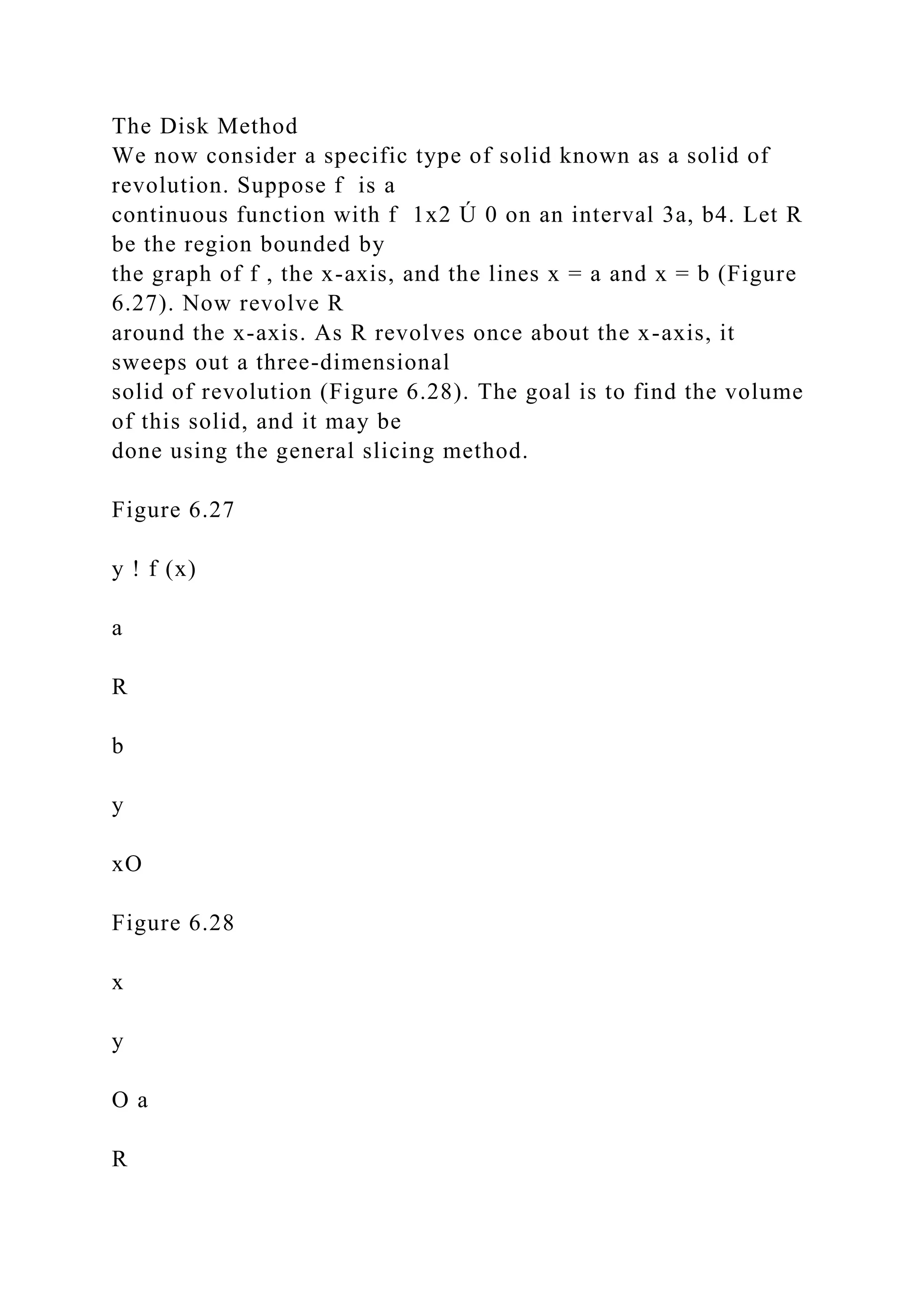
Figure 6.71
y
O xba
y ! F(x)
force
Force varies on [a, b]
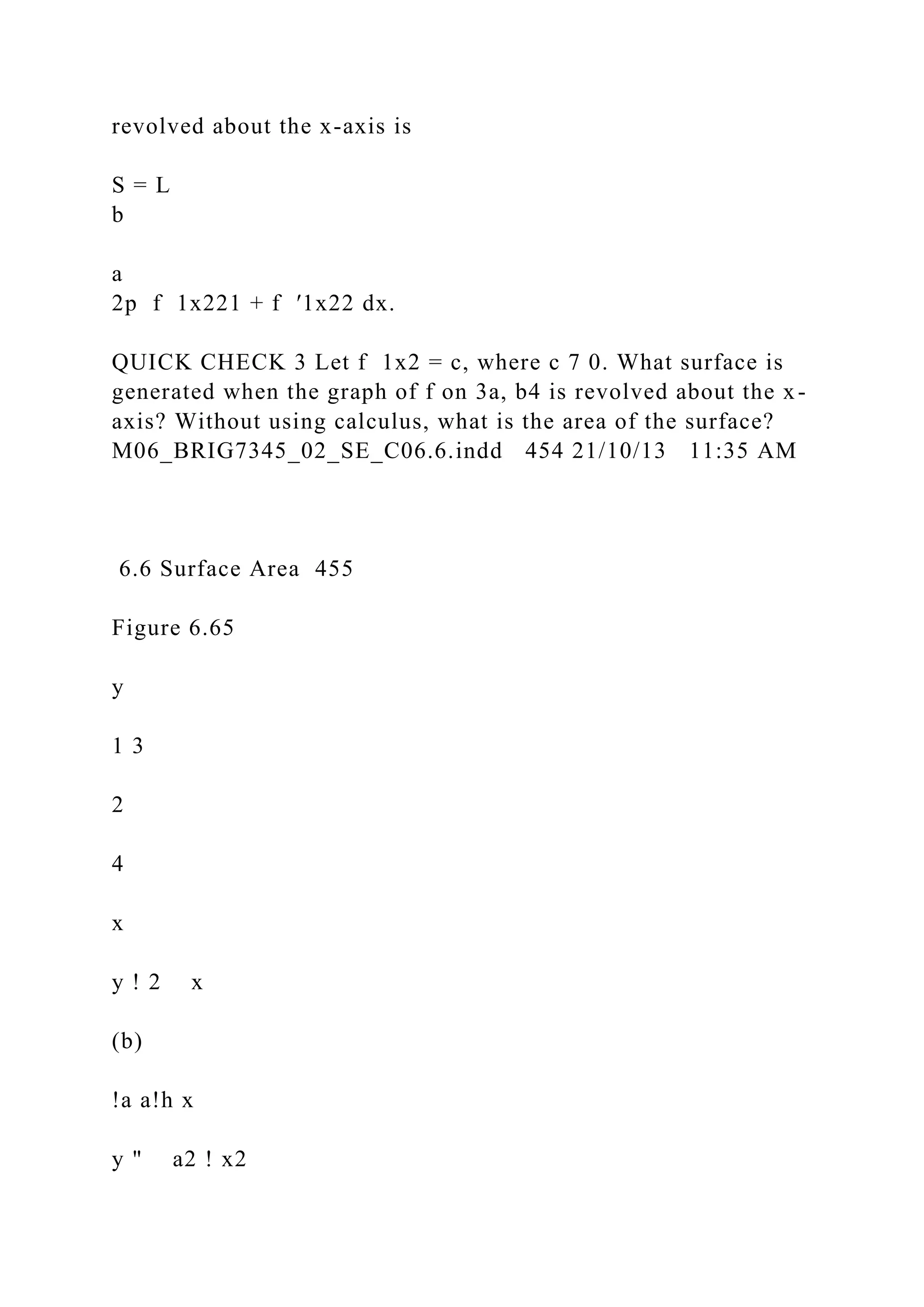
DEFINITION Mass of a One-Dimensional Object
Suppose a thin bar or wire is represented by the interval a … x
… b with a density
function r (with units of mass per length). The mass of the
object is
m = L

b
a
r1x2 dx.
EXAMPLE 1 Mass from variable density A thin 2-m bar,
represented by the interval
0 … x … 2, is made of an alloy whose density in units of kg>m
is given by r1x2 =11 + x22. What is the mass of the bar?
SOLUTION The mass of the bar in kilograms is
m = L
b
a
r1x2 dx = L20 11 + x22 dx = ax + x33 b ` 20 = 143 .
QUICK CHECK 2 A thin bar occupies the interval 0 … x … 2
and has a density in kg>m of
r1x2 = 11 + x22. Using the minimum value of the density, what
is a lower bound for the
mass of the object? Using the maximum value of the density,
what is an upper bound for
the mass of the object?
Work
Work can be described as the change in energy when a force
causes a displacement of an
object. When you carry a basket of laundry up a flight of stairs
or push a stalled car, you
apply a force that results in the displacement of an object, and
work is done. If a constant
force F displaces an object a distance d in the direction of the
force, the work done is the

force multiplied by the distance:
work = force # distance.
It is easiest to use metric units for force and work. A newton
1N2 is the force required to
give a 1-kg mass an acceleration of 1 m>s2. A joule 1J2 is 1
newton-meter [email protected], the
work done by a 1-N force over a distance of 1 m.
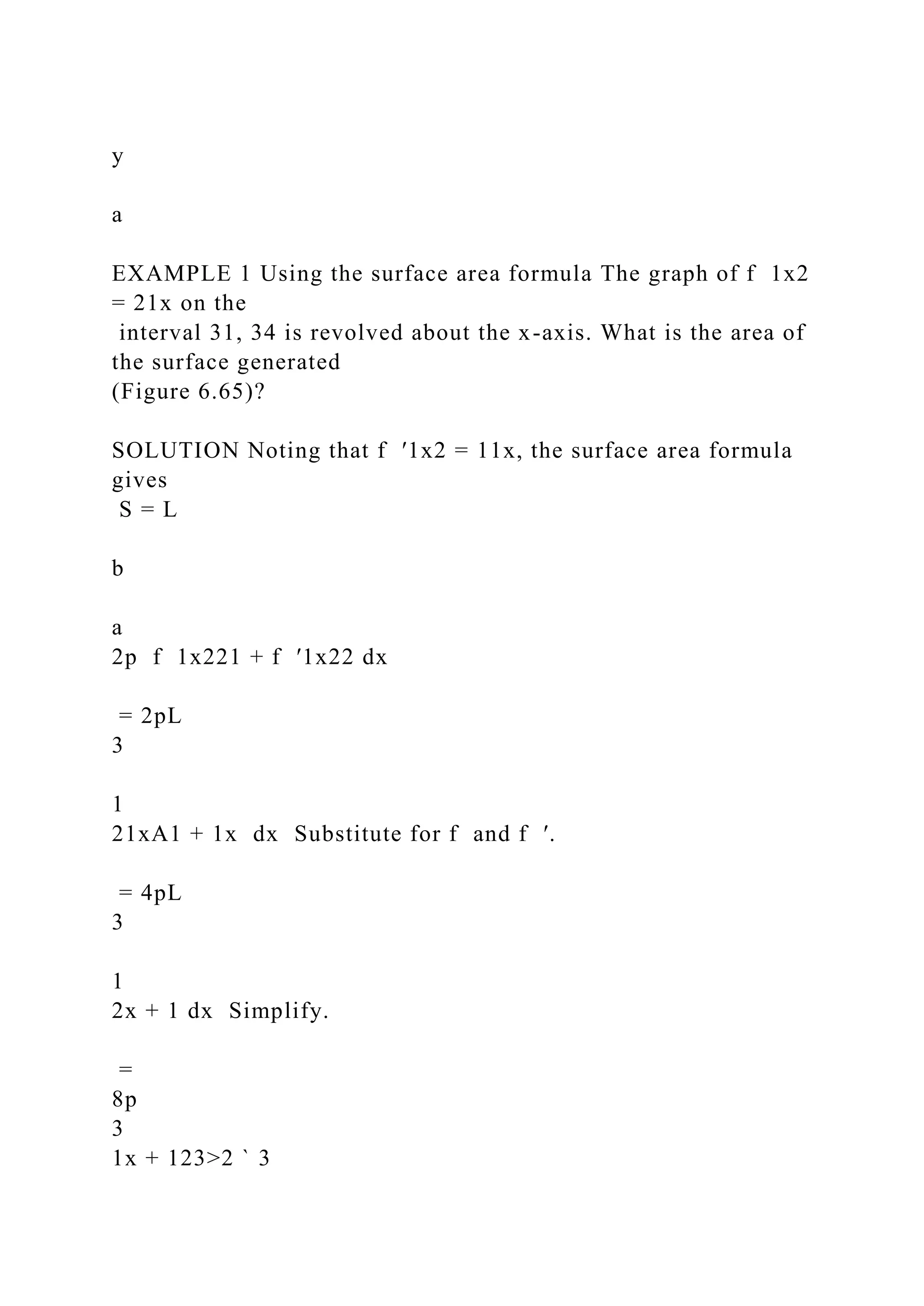
Calculus enters the picture with variable forces. Suppose an
object is moved along
the x-axis by a variable force F that is directed along the x-axis
(Figure 6.71). How much
work is done in moving the object between x = a and x = b?
Once again, we use the
slice-and-sum strategy.
The interval 3a, b4 is divided into n subintervals of equal length
∆x = 1b - a2>n.
We let xk
* be any point in the kth subinterval, for k = 1, c, n. On that
subinterval, the
force is approximately constant with a value of F 1xk*2.
Therefore, the work done in mov-
ing the object across the kth subinterval is approximately F
1xk*2∆x 1force # distance2.
Summing the work done over each of the n subintervals, the
total work over the interval 3a, b4 is approximately
W ≈ a
n
k = 1
F 1xk*2∆x.

This approximation becomes exact when we take the limit as n
S ∞ and ∆x S 0.
The total work done is the integral of the force over the interval
3a, b4 (or, equivalently,
the net area under the force curve in Figure 6.71).
M06_BRIG7345_02_SE_C06.7-6.8.indd 460 21/10/13 11:35
AM
An application of force and work that is easy to visualize is the
stretching and com-
pression of a spring. Suppose an object is attached to a spring
on a frictionless horizontal
surface; the object slides back and forth under the influence of
the spring. We say that the
spring is at equilibrium when it is neither compressed nor
stretched. It is convenient to let
x be the position of the object, where x = 0 is the equilibrium
position (Figure 6.72).
Figure 6.72
Compressed
Equilibrium
Stretched
x ! 0
x " 0

F " 0
x ! 0
x ! 0x # 0
F # 0
Figure 6.73
F
x
F(x) ! kx
Spring is
compressed.
Spring is
stretched.
DEFINITION Work
The work done by a variable force F moving an object along a
line from x = a to
x = b in the direction of the force is
W = L
b
a
F 1x2 dx.
QUICK CHECK 3 Explain why the sum of the work over n
subintervals is only an approxi-
mation of the total work.

According to Hooke’s law, the force required to keep the spring
in a compressed or
stretched position x units from the equilibrium position is F
1x2 = kx, where the positive
spring constant k measures the stiffness of the spring. Note that
to stretch the spring to
a position x 7 0, a force F 7 0 (in the positive direction) is
required. To compress the
spring to a position x 6 0, a force F 6 0 (in the negative
direction) is required (Figure 6.73).
In other words, the force required to displace the spring is
always in the direction of the
displacement.
EXAMPLE 2 Compressing a spring Suppose a force of 10 N is
required to stretch a
spring 0.1 m from its equilibrium position and hold it in that
position.
a. Assuming that the spring obeys Hooke’s law, find the spring
constant k.
b. How much work is needed to compress the spring 0.5 m from
its equilibrium position?
c. How much work is needed to stretch the spring 0.25 m from
its equilibrium position?
d. How much additional work is required to stretch the spring
0.25 m if it has already
been stretched 0.1 m from its equilibrium position?
SOLUTION
a. The fact that a force of 10 N is required to keep the spring
stretched at x = 0.1 m
means (by Hooke’s law) that F 10.12 = k10.1 m2 = 10 N.

Solving for the spring
constant, we find that k = 100 N>m. Therefore, Hooke’s law for
this spring is
F 1x2 = 100x.
b. The work in joules required to compress the spring from x =
0 to x = -0.5 is
W = L
b
a
F 1x2 dx = L -0.50 100x dx = 50x2 ` -0.50 = 12.5.
➤ Hooke’s law was proposed by the English
scientist Robert Hooke (1635–1703),
who also coined the biological term cell.
Hooke’s law works well for springs made
of many common materials. However,
some springs obey more complicated
spring laws (see Exercise 51).
M06_BRIG7345_02_SE_C06.7-6.8.indd 461 21/10/13 11:36
AM
Figure 6.74
y
x
!y

yn " b
yn#1
yk
yk#1
y2
y1
yk*
y0 " 0
h # yk*
y " h (outflow level)
Work to lift kth layer
! A(yk*) !y !g $ (h # yk*)
Work to lift all layers
!
k"1
n
% A(yk*) !y !g $ (h # yk*)
h
Volume of kth layer

! A(yk*) !y
Force on kth layer
! A(yk*) !y $ ! $ g
The kth layer occupying the interval 3yk - 1, yk4, for k = 1, c,
n, is approximately yk*
units above the bottom of the tank, where yk
* is any point in 3yk - 1, yk4.
The cross-sectional area of the kth layer at yk
*, denoted A1yk*2, is determined by
the shape of the tank; the solution depends on being able to find
A for all values of y.
Because the volume of the kth layer is approximately
A1yk*2∆y, the force on the kth layer
(its weight) is
mass
t
Fk = mg ≈ A1yk*2∆y # r # g.
t 6
volume density
To reach the level y = h, the kth layer is lifted an approximate
distance 1h - yk*2
(Figure 6.74). So the work in lifting the kth layer to a height h
is approximately
Wk = A1yk*2∆yrg # 1h - yk*2.
force distance
Summing the work required to lift all the layers to a height h,

the total work is
W ≈ a
n
k = 1
Wk = a
n
k = 1
A1yk*2rg1h - yk*2∆y.
This approximation becomes more accurate as the width of the
layers ∆y tends to
zero and the number of layers tends to infinity. In this limit, we
obtain a definite integral
from y = 0 to y = b. The total work required to empty the tank is
W = lim
nS ∞ a
n
k = 1
A1yk*2rg1h - yk*2∆y = Lb0 rgA1y21h - y2 dy.
This derivation assumes that the bottom of the tank is at y = 0,
in which case the
distance that the slice at level y must be lifted is D1y2 = h - y.
If you choose a different
location for the origin, the function D will be different. Here is
a general procedure for any
choice of origin.
➤ The choice of a coordinate system is

somewhat arbitrary and may depend on
the geometry of the problem. You can let
the y-axis point upward or downward,
and there are usually several logical
choices for the location of y = 0.
You should experiment with different
coordinate systems.
c. The work in joules required to stretch the spring from x = 0
to x = 0.25 is
W = L
b
a
F 1x2 dx = L0.250 100x dx = 50x2 ` 0.250 = 3.125.
d. The work in joules required to stretch the spring from x = 0.1
to x = 0.35 is
W = L
b
a
F 1x2 dx = L0.350.1 100x dx = 50x2 ` 0.350.1 = 5.625.
Comparing parts (c) and (d), we see that more work is required
to stretch the spring 0.25 m
starting at x = 0.1 than starting at x = 0. Related Exercises 17–
26
Lifting Problems Another common work problem arises when
the motion is vertical and
the force is the gravitational force. The gravitational force
exerted on an object with mass m
is F = mg, where g ≈ 9.8 m>s2 is the acceleration due to gravity

near the surface of Earth.
The work in joules required to lift an object of mass m a
vertical distance of y meters is
work = force # distance = mgy.
This type of problem becomes interesting when the object being
lifted is a body of
water, a rope, or a chain. In these situations, different parts of
the object are lifted different
distances—so integration is necessary. Here is a typical
situation and the strategy used.
Suppose a fluid such as water is pumped out of a tank to a
height h above the bottom
of the tank. How much work is required, assuming the tank is
full of water? Three key
observations lead to the solution.
Water from different levels of the tank is lifted different
vertical distances, requiring
different amounts of work.
Two equal volumes of water from the same horizontal plane are
lifted the same distance
and require the same amount of work.
A volume V of water has mass rV, where r = 1 g>cm3 = 1000
kg>m3 is the density of
water.
To solve this problem, we let the y-axis point upward with y = 0
at the bottom of the
tank. The body of water that must be lifted extends from y = 0
to y = b (which may be
the top of the tank). The level to which the water must be raised

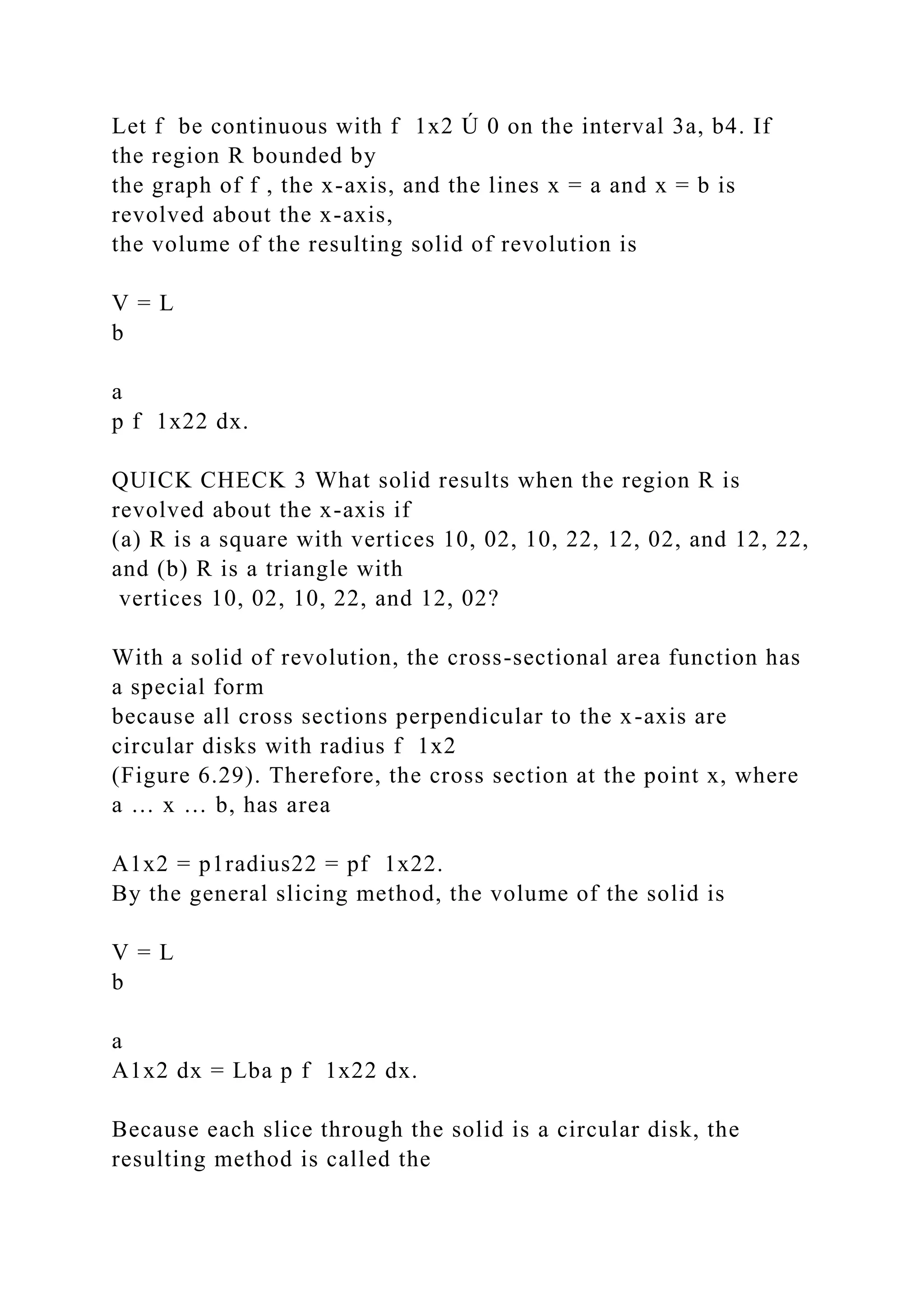
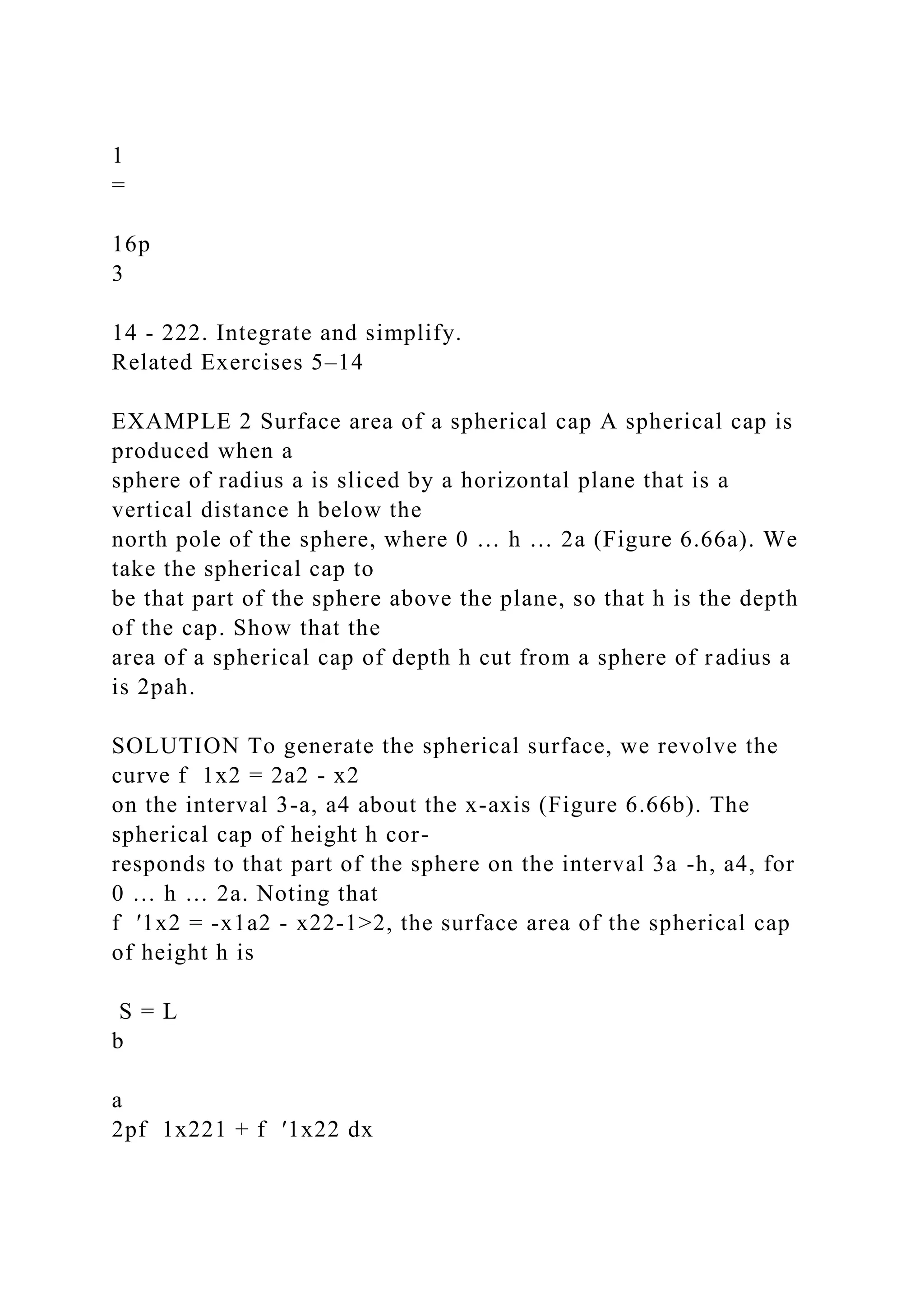
is y = h, where h Ú b
(Figure 6.74). We now slice the water into n horizontal layers,
each having thickness ∆y.
➤ Notice again that the units in the integral
are consistent. If F has units of N and x
has units of m, then W has units of F dx,
or [email protected], which are the units of work 11
[email protected] = 1 J2.
QUICK CHECK 4 In Example 2, explain
why more work is needed in part
(d) than in part (c), even though the
displacement is the same.
M06_BRIG7345_02_SE_C06.7-6.8.indd 462 21/10/13 11:36
AM
PROCEDURE Solving Lifting Problems
1. Draw a y-axis in the vertical direction (parallel to gravity)
and choose a con-
venient origin. Assume the interval 3a, b4 corresponds to the
vertical extent of
the fluid.
2. For a … y … b, find the cross-sectional area A1y2 of the
horizontal slices and
the distance D1y2 the slices must be lifted.
3. The work required to lift the water is

W = L
b
a
rgA1y2D1y2 dy.
The kth layer occupying the interval 3yk - 1, yk4, for k = 1, c,
n, is approximately yk*
units above the bottom of the tank, where yk
* is any point in 3yk - 1, yk4.
The cross-sectional area of the kth layer at yk
*, denoted A1yk*2, is determined by
the shape of the tank; the solution depends on being able to find
A for all values of y.
Because the volume of the kth layer is approximately
A1yk*2∆y, the force on the kth layer
(its weight) is
mass
t
Fk = mg ≈ A1yk*2∆y # r # g.
t 6
volume density
To reach the level y = h, the kth layer is lifted an approximate
distance 1h - yk*2
(Figure 6.74). So the work in lifting the kth layer to a height h
is approximately
Wk = A1yk*2∆yrg # 1h - yk*2.
force distance
Summing the work required to lift all the layers to a height h,

somewhat arbitrary and may depend on
the geometry of the problem. You can let
the y-axis point upward or downward,
and there are usually several logical
choices for the location of y = 0.
You should experiment with different
coordinate systems.
t t
We now use this procedure to solve two pumping problems.
EXAMPLE 3 Pumping water How much work is needed to pump
all the water out of
a cylindrical tank with a height of 10 m and a radius of 5 m?
The water is pumped to an
outflow pipe 15 m above the bottom of the tank.
M06_BRIG7345_02_SE_C06.7-6.8.indd 463 21/10/13 11:36
AM
SOLUTION In this problem, we choose a different origin by
letting y = 0 and y = -5
correspond to the center and the bottom of the tank,
respectively. For -5 … y … 0, a hori-
zontal layer of gasoline located at a depth y is a rectangle with
a length of 10 and width of
2225 - y2 (Figure 6.76). Therefore, the cross-sectional area of
the layer at depth y is
A1y2 = 20225 - y2.
➤ Again, there are several choices for the

location of the origin. The location in this
example makes A1y2 easy to compute.
SOLUTION Figure 6.75 shows the cylindrical tank filled to
capacity and the outflow 15 m
above the bottom of the tank. We let y = 0 represent the bottom
of the tank and y = 10
represent the top of the tank. In this case, all horizontal slices
are circular disks of radius
r = 5 m. Therefore, for 0 … y … 10, the cross-sectional area is
A1y2 = pr2 = p52 = 25p.
Note that the water is pumped to a level h = 15 m above the
bottom of the tank, so the
lifting distance is D1y2 = 15 - y. The resulting work integral is
W = L
10
0
rgA1y2 D1y2 dy = 25prgL100 115 - y2 dy.
25p 15 - y
Substituting r = 1000 kg>m3 and g = 9.8 m>s2, the total work
in joules is
W = 25prgL
10
0
115 - y2 dy
= 25p11000219.82a15y - 1
2

y2b ` 10
0
r g
≈ 7.7 * 107.
The work required to pump the water out of the tank is
approximately 77 million joules.
QUICK CHECK 5 In the previous example, how would the
integral change if the outflow
pipe were at the top of the tank?
EXAMPLE 4 Pumping gasoline A cylindrical tank with a length
of 10 m and a radius
of 5 m is on its side and half-full of gasoline (Figure 6.76).
How much work is required
to empty the tank through an outlet pipe at the top of the tank?
1The density of gasoline is
r ≈ 737 kg>m3.2
➤ Recall that g ≈ 9.8 m>s2. You should
verify that the units are consistent in this
calculation: The units of r, g, A1y2, D1y2,
and dy are kg>m3, m>s2, m2, m, and m,
respectively. The resulting units of W are
kg m2>s2, or J. A more convenient unit
for large amounts of work and energy is
the kilowatt-hour, which is 3.6 million
joules.
e e
eFigure 6.75

r ! 5
y ! 15 (outflow level)
y ! 10
(tank top)
y ! water
layer level
y ! 0
(bottom)
15 " y !
distance water
layer is lifted
y
x
The area of
water layer is
A(y) ! !(52).
!r2
Figure 6.76
y
length ! 10
D(y) ! 5 " y

y ! "5
y ! 0
2. ... the width of the gasoline
layer is 2 25 " y2.
3. The area of the gasoline layer
is A(y) ! 10 # 2 25 " y2.
1. Because this width
is 25 " y2...
y5
!5
5!5
The equation of the
right side of the
circle is x " 25 ! y2.
y
x
M06_BRIG7345_02_SE_C06.7-6.8.indd 464 21/10/13 11:36
AM
Figure 6.77

w(y)a ! yk*
y " 0
y " a
Pressure on strip
! !g(a ! yk*)
Force on strip
! !g(a ! yk*) # area of strip
! !g(a ! yk*) w(yk*) $y
$y yk*
yk!1
yk
y
The distance the layer at level y must be lifted to reach the top
of the tank is D1y2 = 5 - y,
where 5 … D1y2 … 10. The resulting work integral is
W = 73719.82L0-5 20225 - y2 15 - y2 dy = 144,452L0-5 225 -
y2 15 - y2 dy.
r g A1y2 D1y2
This integral is evaluated by splitting the integrand into two
pieces and recognizing that
one piece is the area of a quarter circle of radius 5:
L
0
-5

225 - y2 15 - y2 dy = 5L0-5 225 - y2 dy - L0-5y225 - y2 dy
area of quarter circle let u = 25 - y2; du = -2y dy
= 5 # 25p
4
+ 1
2 L
25
0
1u du
=
125p
4
+ 1
3
u3>2 `
0
25
=
375p + 500
12
.
Multiplying this result by 20 rg = 144,452, we find that the
work required is approxi-

mately 20.2 million joules. Related Exercises 27–37
Force and Pressure
Another application of integration deals with the force exerted
on a surface by a body of
water. Again, we need a few physical principles.
Pressure is a force per unit area, measured in units such as
newtons per square
meter 1N>m22. For example, the pressure of the atmosphere on
the surface of Earth is
about 14 lb>in2 1approximately 100 kilopascals, or 105 N>m22.
As another example, if
you stood on the bottom of a swimming pool, you would feel
pressure due to the weight
(force) of the column of water above your head. If your head is
flat and has surface area
A m2 and it is h meters below the surface, then the column of
water above your head has
volume Ah m3. That column of water exerts a force (its weight)
F = mass # acceleration = volume # density # g = Ahrg,
mass
where r is the density of water and g is the acceleration due to
gravity. Therefore, the
pressure on your head is the force divided by the surface area of
your head:
pressure =
force
A
=
Ahrg

A
= rgh.
This pressure is called hydrostatic pressure (meaning the
pressure of water at rest),
and it has the following important property: It has the same
magnitude in all directions.
Specifically, the hydrostatic pressure on a vertical wall of the
swimming pool at a depth
h is also rgh. This is the only fact needed to find the total force
on vertical walls such as
dams. We assume that the water completely covers the face of
the dam.
The first step in finding the force on the face of the dam is to
introduce a coordinate
system. We choose a y-axis pointing upward with y = 0
corresponding to the base of the
dam and y = a corresponding to the top of the dam (Figure
6.77). Because the pressure
varies with depth (y-direction), the dam is sliced horizontally
into n strips of equal thick-
ness ∆y. The kth strip corresponds to the interval 3yk - 1, yk4,
and we let yk* be any point in
that interval. The depth of that strip is approximately h = a -
yk*, so the hydrostatic pres-
sure on that strip is approximately rg1a - yk*2.
The crux of any dam problem is finding the width of the strips
as a function of y,
which we denote w1y2. Each dam has its own width function;
however, once the width
function is known, the solution follows directly. The
approximate area of the kth strip is

e e g c
i i
h
M06_BRIG7345_02_SE_C06.7-6.8.indd 465 21/10/13 11:36
AM
EXAMPLE 5 Force on a dam A large vertical dam in the shape
of a symmetric
trapezoid has a height of 30 m, a width of 20 m at its base, and
a width of 40 m at the top
(Figure 6.78). What is the total force on the face of the dam
when the reservoir is full?
SOLUTION We place the origin at the center of the base of the
dam (Figure 6.79). The
right slanted edge of the dam is a segment of the line that
passes through the points 110, 02 and 120, 302. An equation of
that line is
y - 0 = 30
10
1x - 102 or y = 3x - 30 or x = 1
3
1y + 302.
Notice that at a depth of y, where 0 … y … 30, the width of the
dam is
w1y2 = 2x = 2

3
1y + 302.➤ You should check the width function: w102 = 20
(the width of the dam at its base) and w1302 = 40 (the width of
the
dam at its top).
its width multiplied by its thickness, or w1yk*2∆y. The force on
the kth strip (which is the
area of the strip multiplied by the pressure) is approximately
Fk = rg1a - yk*2w1yk*2∆y.
pressure area of strip
Summing the forces over the n strips, the total force is
F ≈ a
n
k = 1
Fk = a
n
k = 1
rg1a - yk*2w1yk*2∆y.
To find the exact force, we let the thickness of the strips tend to
zero and the number
of strips tend to infinity, which produces a definite integral. The
limits of integration cor-
respond to the base 1y = 02 and top 1y = a2 of the dam.
Therefore, the total force on the
dam is
F = lim

nS ∞ a
n
k = 1
rg1a - yk*2w1yk*2∆y = La0 rg1a - y2w1y2 dy.
➤ We have chosen y = 0 to be the base of
the dam. Depending on the geometry of
the problem, it may be more convenient
(less computation) to let y = 0 be at the
top of the dam. Experiment with different
choices.
d d
PROCEDURE Solving Force Problems
1. Draw a y-axis on the face of the dam in the vertical direction
and choose a
convenient origin (often taken to be the base of the dam).
2. Find the width function w1y2 for each value of y on the face
of the dam.
3. If the base of the dam is at y = 0 and the top of the dam is at
y = a, then the
total force on the dam is
F = L
a
0
rg1b - y2w1y2 dy.
depth width

ed
Figure 6.78
40
20
30
Figure 6.79
!30 0
y
x
40
(20, 30)
y " 3x ! 30
x " W(y # 30)
w(y) " (y # 30)
(10, 0)
M06_BRIG7345_02_SE_C06.7-6.8.indd 466 21/10/13 11:36
AM
6.8 Logarithmic and Exponential Functions Revisited 471

6.8 Logarithmic and Exponential
Functions Revisited
Earlier in the text, we made several claims about exponential
and logarithmic functions,
but we did not prove them. (For example, these functions are
continuous and differen-
tiable on their domains.) Our objective in this section is to
place these important functions
on a solid foundation by presenting a more rigorous
development of their properties.
Before embarking on this program, we offer a roadmap to help
guide you through the
section. We carry out the following four steps.
1. We first define the natural logarithm function in terms of an
integral, and then derive
the properties of ln x directly from this new definition.
60. Orientation and force A plate shaped like an equilateral
triangle
1 m on a side is placed on a vertical wall 1 m below the surface
of
a pool filled with water. On which plate in the figure is the
force
greater? Try to anticipate the answer and then compute the force
on each plate.
surface
1 m
surface

1 m
1 m
1 m
61. Orientation and force A square plate 1 m on a side is placed
on a
vertical wall 1 m below the surface of a pool filled with water.
On
which plate in the figure is the force greater? Try to anticipate
the
answer and then compute the force on each plate.
surface
1 m
1 m
1 m
surface
1 m
62. A calorie-free milkshake? Suppose a cylindrical glass with a
diameter of 112 m and a height of
1
10 m is filled to the brim with a
400-Cal milkshake. If you have a straw that is 1.1 m long (so
the
top of the straw is 1 m above the top of the glass), do you burn
off
all the calories in the milkshake in drinking it? Assume that the

density of the milkshake is 1 g>cm3 11 Cal = 4184 J2.
63. Critical depth A large tank has a plastic window on one wall
that
is designed to withstand a force of 90,000 N. The square
window
is 2 m on a side, and its lower edge is 1 m from the bottom of
the
tank.
a. If the tank is filled to a depth of 4 m, will the window
withstand the resulting force?
b. What is the maximum depth to which the tank can be filled
without the window failing?
64. Buoyancy Archimedes’ principle says that the buoyant force
ex-
erted on an object that is (partially or totally) submerged in
water
is equal to the weight of the water displaced by the object (see
figure). Let rw = 1 g>cm3 = 1000 kg>m3 be the density of
water
and let r be the density of an object in water. Let f = r>rw. If
0 6 f … 1, then the object floats with a fraction f of its volume
submerged; if f 7 1, then the object sinks.
buoyant force
volume of
displaced water
Consider a cubical box with sides 2 m long floating in water
with one-half of its volume submerged 1r = rw>22. Find the
force required to fully submerge the box (so its top surface is at
the water level).

(See the Guided Project Buoyancy and Archimedes’ Principle
for
further explorations of buoyancy problems.)
QUICK CHECK ANSWERS
1. a. The bar is heaviest at the left end and lightest at the
right end. b. r = 2.5 g>cm. 2. Minimum mass = 2 kg;
maximum mass = 10 kg 3. We assume that the force is
constant over each subinterval, when, in fact, it varies over
each subinterval. 4. The restoring force of the spring in-
creases as the spring is stretched 1 f 1x2 = 100x2. Greater
restoring forces are encountered on the interval 30.1, 0.354
than on the interval 30, 0.254. 5. The factor 115 - y2 in
the integral is replaced with 110 - y2.
M06_BRIG7345_02_SE_C06.7-6.8.indd 471 21/10/13 11:36
AM
All the familiar geometric and algebraic properties of the
natural logarithmic function fol-
low directly from this new integral definition.
Properties of the Natural Logarithm
Domain, range, and sign Because the natural logarithm is
defined as a definite integral,
its value is the net area under the curve y = 1>t between t = 1
and t = x. The integrand
is undefined at t = 0, so the domain of ln x is 10, ∞2. On the
interval 11, ∞2, ln x is
positive because the net area of the region under the curve is

positive (Figure 6.80a). On 10, 12, we have L x1 1t dt = - L1x
1t dt, which implies ln x is negative (Figure 6.80b). As
expected, when x = 1, we have ln 1 = L
1
1
1
t
dt = 0. The net area interpretation of ln x
also implies that the range of ln x is 1- ∞ , ∞2 (see Exercise 72
for an outline of a proof).
2. The natural exponential function ex is introduced as the
inverse of ln x, and the prop-
erties of ex are developed by appealing to this inverse
relationship. We also present
derivative and integral formulas associated with these functions.
3. Next, we define the general exponential function bx in terms
of ex, and the general
logarithmic function logb x in terms of ln x. The derivative and
integral results stated in
Section 3.9 follow immediately.
4. Finally, we revisit the General Power Rule (Section 3.9) and
we also derive a limit that
can be used to approximate e.
Step 1: The Natural Logarithm
Our aim is to develop the properties of the natural logarithm
using definite integrals. It all
begins with the following definition.

DEFINITION The Natural Logarithm
The natural logarithm of a number x 7 0, is ln x = L
x
1
1
t
dt.
Figure 6.80
1
(a)
0
y
tx
1
x dt
t
! 0.
If x ! 1,
net area " ln x " !
If 0 # x # 1,
net area " ln x " !

1
x dt
t
# 0.
1
t
y "
1
(b)
0
y
tx
1
t
y "
Derivative The derivative of the natural logarithm follows
immediately from its defini-
tion and the Fundamental Theorem of Calculus:
d
dx
1ln x2 = d
dx L

x
1
dt
t
=
1
x
, for x 7 0.
➤ By the Fundamental Theorem of
Calculus,
d
dx L
x
a
f 1t2 dt = f 1x2.
M06_BRIG7345_02_SE_C06.7-6.8.indd 472 21/10/13 11:36
AM
We have two important consequences.
Because its derivative is defined for x 7 0, ln x is a
differentiable function for x 7 0,
which means it is continuous on its domain (Theorem 3.1).

Because 1>x 7 0 for x 7 0, ln x is strictly increasing and one-to-
one on its domain;
therefore, it has a well-defined inverse.
The Chain Rule allows us to extend the derivative property to
all nonzero real numbers
(Exercise 70). By differentiating ln 1-x2 for x 6 0, we find that
d
dx
1ln ! x !2 = 1
x
, for x ≠ 0.
More generally, by the Chain Rule,
d
dx
1ln ! u1x2 !2 = 1
u1x2 u′1x2 = u′1x2u1x2 .
Graph of ln x As noted before, ln x is continuous and strictly
increasing for x 7 0. The
second derivative,
d2
dx2
1ln x2 = - 1
x2
, is negative for x 7 0, which implies the graph of

ln x is concave down for x 7 0. As demonstrated in Exercise 72,
lim
xS∞
ln x = ∞ , and lim
xS0+
ln x = - ∞ .
This information, coupled with the fact that ln 1 = 0, gives the
graph of y = ln x
(Figure 6.81).
Logarithm of a product The familiar logarithm property
ln xy = ln x + ln y, for x 7 0, y 7 0,
may be proved using the integral definition:
ln xy = L
xy
1
dt
t
Definition of ln xy
= L
x
1

dt
t
+ L
xy
x
dt
t
Additive property of integrals
= L
x
1
dt
t
+ L
y
1
du
u
Substitute u = t>x in second integral.
= ln x + ln y. Definition of ln
Logarithm of a quotient Assuming x 7 0 and y 7 0, the product
property and a bit of
algebra give

ln x = ln ay # x
y
b = ln y + ln x
y
.
Solving for ln 1x>y2, we have
ln
x
y
= ln x - ln y,
which is the quotient property for logarithms.
QUICK CHECK 1 What is the domain of
ln ! x !?
Figure 6.81
0
y
x
y ! ln x
(1, 0)
lim ln x ! "
lim ln x ! #"

x!"
x!0
$
d2
dx2
(ln x) % 0 !& concave down
d
dx
(ln x) & 0 !& ln x is increasing for x > 0
M06_BRIG7345_02_SE_C06.7-6.8.indd 473 21/10/13 11:36
AM
EXAMPLE 1 Integrals with ln x Evaluate L
4
0
x
x2 + 9
dx.
SOLUTION
L
4

0
x
x2 + 9
dx =
1
2 L
25
9
du
u
Let u = x2 + 9; du = 2x dx.
=
1
2
ln ! u ! `
9
25
Fundamental Theorem
=
1
2
1ln 25 - ln 92 Evaluate.

= ln
5
3
Properties of logarithms
Logarithm of a power Assuming x 7 0 and p is rational, we have
ln xp = L
xp
1
dt
t
Definition of ln xp
= pL
x
1
du
u
Let t = up; dt = pup - 1du.
= p ln x. By definition, ln x = L
x
1

du
u
.
This argument relies on the Power Rule 1dt = pup - 1 du2,
which we proved only for ratio-
nal exponents. Later in this section, we prove that ln xp = p ln
x, for all real values of p.
Integrals Because
d
dx
1ln ! x !2 = 1
x
, we have
L
1
x
dx = ln ! x ! + C.
We have shown that the familiar properties of ln x follow from
its new integral definition.
THEOREM 6.4 Properties of the Natural Logarithm
1. The domain and range of ln x are 10, ∞2 and 1- ∞ , ∞2,
respectively.
2. ln xy = ln x + ln y, for x 7 0 and y 7 0
3. ln 1x>y2 = ln x - ln y, for x 7 0 and y 7 0
4. ln xp = p ln x, for x 7 0 and p a rational number

5.
d
dx
1ln ! x !2 = 1
x
, for x ≠ 0
6.
d
dx
1ln ! u1x2 !2 = u′1x2
u1x2 , for u1x2 ≠ 0
7. L
1
x
dx = ln ! x ! + C
M06_BRIG7345_02_SE_C06.7-6.8.indd 474 21/10/13 3:14
PM
The number e has the property that the area of the region
bounded by the graph of
y =
1
t
and the t-axis on the interval 31, e4 is 1 (Figure 6.83). Note
that ln 2 6 1 and

ln 3 7 1 (Exercise 73). Because ln x is continuous on its domain,
the Intermediate Value
Theorem ensures that there is a number e with 2 6 e 6 3 such
that ln e = 1.
Step 2: The Exponential Function
We have established that f 1x2 = ln x is a continuous,
increasing function on the interval 10, ∞2. Therefore, it is one-
to-one and its inverse function exists on 10, ∞2. We denote
the inverse function f -11x2 = exp 1x2. Its graph is obtained by
reflecting the graph of
f 1x2 = ln x about the line y = x (Figure 6.82). The domain of
exp 1x2 is 1- ∞ , ∞2 be-
cause the range of ln x is 1- ∞ , ∞2, and the range of exp 1x2 is
10, ∞2 because the domain
of ln x is 10, ∞2.
The usual relationships between a function and its inverse also
hold:
y = exp 1x2 if and only if x = ln y;
exp 1ln x2 = x, for x 7 0, and ln 1exp 1x22 = x, for all x.
We now appeal to the properties of ln x and use the inverse
relations between ln x and
exp 1x2 to show that exp 1x2 satisfies the expected properties
of any exponential func-
tion. For example, if x1 = ln y1 and x2 = ln y2, then it follows
that y1 = exp 1x12,
y2 = exp 1x22, and
exp 1x1 + x22 = exp 1ln y1 + ln y22 Substitute x1 = ln y1, x2 =
ln y2.
ln y1y2

= exp 1ln y1y22 Properties of logarithms
= y1y2 Inverse property of exp 1x2 and ln x
= exp 1x12 exp 1x22. y1 = exp 1x12, y2 = exp 1x22
Therefore, exp 1x2 satisfies the property of exponential
functions bx1 + x2 = bx1bx2. Similar
arguments show that exp 1x2 satisfies other characteristic
properties of exponential func-
tions ( Exercise 71):
exp 102 = 1,
exp 1x1 - x22 = exp 1x12exp 1x22, and
1exp 1x22p = exp 1px2, for rational numbers p.
Suspecting that exp 1x2 is an exponential function, the next task
is to identify its base.
Let’s consider the real number exp (1), and with a bit of
forethought, call it e. The inverse
relationship between ln x and exp 1x2 implies that
if e = exp 112, then ln e = ln 1exp 1122 = 1.
Using the fact that ln e = 1 and the integral definition of ln x,
we now formally define e.
g
DEFINITION The Number e
The number e is the real number that satisfies ln e = L
e
1
dt
t

= 1.
Figure 6.82
42 x
4
2
y
y ! x
y ! ln x
domain (0, ")
range (#", ")
y ! exp(x)
domain (#", ")
range (0, ")
Figure 6.83
0
y
t3e21
1
t
y !
ln 2 " 1 ln 3 # 1

dt
tln e ! ! ! 1
area ! ln e ! 1
1
e
➤ We give a limit definition that provides a
good approximation to e at the end of this
section.
M06_BRIG7345_02_SE_C06.7-6.8.indd 475 21/10/13 11:36
AM
We may now dispense with the notation exp 1x2 and use ex as
the inverse of ln x. The
usual inverse relationships between ex and ln x hold, and the
properties of exp 1x2 can now
be written for ex.
DEFINITION The Exponential Function
For any real number x, y = ex = exp 1x2, where x = ln y.
We can now show that indeed exp 1x2 is the exponential
function ex. Assume that p is
a rational number and note that ep 7 0. By property 4 of
Theorem 6.4 we have
ln ep = p ln e = p.
1

Using the inverse relationship between ln x and exp 1x2, we
also know that
ln exp 1p2 = p.
Equating these two expressions for p, we conclude that ln e p =
ln exp 1p2. Because ln x is
a one-to-one function, it follows that
ep = exp 1p2, for rational numbers p,
and we conclude that exp (x) is the exponential function with
base e.
We already know how to evaluate ex when x is rational. For
example, e3 = e # e # e,
e-2 =
1
e # e, and e1>2 = 1e. But how do we evaluate ex when x is
irrational? We proceed
as follows. The function x = ln y is defined for y 7 0 and its
range is all real numbers.
Therefore, the domain of its inverse y = exp 1x2 is all real
numbers; that is, exp 1x2 is de-
fined for all real numbers. We now define ex to be exp 1x2
when x is irrational.
THEOREM 6.5 Properties of ex
The exponential function ex satisfies the following properties,
all of which result
from the integral definition of ln x. Let x and y be real numbers.
1. ex + y = exey

2. ex - y = ex>ey
3. 1ex2p = exp, where p is a rational number
4. ln 1ex2 = x
5. eln x = x, for x 7 0
➤ The restriction on p in property 3 will be
lifted shortly.
QUICK CHECK 2 Simplify eln 2x, ln 1e2x2, e2 ln x, and ln
12ex2.
Derivatives and Integrals By Theorem 3.23 (derivatives of
inverse functions), the
derivative of the exponential function exists for all x. To
compute
d
dx
1ex2, we observe that
ln 1ex2 = x and then differentiate both sides with respect to x:
d
dx
1ln ex2 = d
dx
1x2
1
1
ex
d

dx
1ex2 = 1 d
dx
1ln u1x22 = u′1x2
u1x2 (Chain Rule)
d
dx
1ex2 = ex. Solve for d
dx
1ex2.
e
c
M06_BRIG7345_02_SE_C06.7-6.8.indd 476 21/10/13 11:36
AM
Once again, we obtain the remarkable result that the exponential
function is its own deriva-
tive. It follows that ex is its own antiderivative up to a constant;
that is,
Lex dx = ex + C.
Extending these results using the Chain Rule, we have the
following theorem.

EXAMPLE 2 Integrals with ex Evaluate L
ex
1 + ex dx.
SOLUTION The change of variables u = 1 + ex implies du = ex
dx:
L
1
1 + ex e
x dx = L
1
u
du u = 1 + ex, du = ex dx
u
du
= ln ! u ! + C Antiderivative of u-1
= ln 11 + ex2 + C. Replace u with 1 + ex.
Note that the absolute value may be removed from ln ! u !
because 1 + ex 7 0, for all x.
Step 3: General Logarithmic and Exponential Functions
We now turn to exponential and logarithmic functions with a
general positive base b. The
first step is to define the exponential function bx for positive
bases with b ≠ 1 and for
all real numbers x. We use property 3 of Theorem 6.5 and the

fact that b = eln b. If x is a
rational number, then
bx = 1eln b2x = ex ln b;
b
this important relationship expresses bx in terms of ex. Because
ex is defined for all real x,
we use this relationship to define bx for all real x.
DEFINITION Exponential Functions with General Bases
Let b be a positive real number with b ≠ 1. Then for all real x,
bx = ex ln b.
QUICK CHECK 3 What is the slope of
the curve y = ex at x = ln 2? What
is the area of the region bounded by
the graph of y = ex and the x-axis
between x = 0 and x = ln 2?
THEOREM 6.6 Derivative and Integral of the Exponential
Function
For real numbers x,
d
dx
1eu1x22 = eu1x2u′1x2 and Lex dx = ex + C.
ee
c
This definition fills the gap in property 4 of Theorem 6.4 1ln xp
= p ln x2. We use the

definition of bx to write
xp = ep ln x, for x 7 0 and p real.
Taking the natural logarithm of both sides and using the inverse
relationship between ex
and ln x, we find that
ln xp = ln ep ln x = p ln x, for x 7 0 and p real.
In this way, we extend property 4 of Theorem 6.4 to real
powers.
Just as bx is defined in terms of ex, logarithms with base b 7 1
and b ≠ 1 may be
expressed in terms of ln x. All that is needed is the change of
base formula (Section 1.3)
logb x =
ln x
ln b
.
➤ Knowing that ln xp = p ln x for real p,
we can also extend property 3 of
Theorem 6.5 to real numbers. For real
x and y, we take the natural logarithm
of both sides of z = 1ex2y, which
gives ln z = y ln ex = xy, or z = exy.
Therefore, 1ex2y = exy.
M06_BRIG7345_02_SE_C06.7-6.8.indd 477 21/10/13 11:36
AM

Once again, we obtain the remarkable result that the exponential
function is its own deriva-
tive. It follows that ex is its own antiderivative up to a constant;
that is,
Lex dx = ex + C.
Extending these results using the Chain Rule, we have the
following theorem.
EXAMPLE 2 Integrals with ex Evaluate L
ex
1 + ex dx.
SOLUTION The change of variables u = 1 + ex implies du = ex
dx:
L
1
1 + ex e
x dx = L
1
u
du u = 1 + ex, du = ex dx
u
du
= ln ! u ! + C Antiderivative of u-1

= ln 11 + ex2 + C. Replace u with 1 + ex.
Note that the absolute value may be removed from ln ! u !
because 1 + ex 7 0, for all x.
Step 3: General Logarithmic and Exponential Functions
We now turn to exponential and logarithmic functions with a
general positive base b. The
first step is to define the exponential function bx for positive
bases with b ≠ 1 and for
all real numbers x. We use property 3 of Theorem 6.5 and the
fact that b = eln b. If x is a
rational number, then
bx = 1eln b2x = ex ln b;
b
this important relationship expresses bx in terms of ex. Because
ex is defined for all real x,
we use this relationship to define bx for all real x.
DEFINITION Exponential Functions with General Bases
Let b be a positive real number with b ≠ 1. Then for all real x,
bx = ex ln b.
QUICK CHECK 3 What is the slope of
the curve y = ex at x = ln 2? What
is the area of the region bounded by
the graph of y = ex and the x-axis
between x = 0 and x = ln 2?
THEOREM 6.6 Derivative and Integral of the Exponential
Function
For real numbers x,

d
dx
1eu1x22 = eu1x2u′1x2 and Lex dx = ex + C.
ee
c
This definition fills the gap in property 4 of Theorem 6.4 1ln xp
= p ln x2. We use the
definition of bx to write
xp = ep ln x, for x 7 0 and p real.
Taking the natural logarithm of both sides and using the inverse
relationship between ex
and ln x, we find that
ln xp = ln ep ln x = p ln x, for x 7 0 and p real.
In this way, we extend property 4 of Theorem 6.4 to real
powers.
Just as bx is defined in terms of ex, logarithms with base b 7 1
and b ≠ 1 may be
expressed in terms of ln x. All that is needed is the change of
base formula (Section 1.3)
logb x =
ln x
ln b
.

➤ Knowing that ln xp = p ln x for real p,
we can also extend property 3 of
Theorem 6.5 to real numbers. For real
x and y, we take the natural logarithm
of both sides of z = 1ex2y, which
gives ln z = y ln ex = xy, or z = exy.
Therefore, 1ex2y = exy.
M06_BRIG7345_02_SE_C06.7-6.8.indd 477 21/10/13 11:36
AM
Theorems 3.18 and 3.20 give us the derivative results for
exponential and logarithmic
functions with a general base b 7 0. Extending those results
with the Chain Rule, we
have the following derivatives and integrals.
SUMMARY Derivatives and Integrals with Other Bases
Let b 7 0 and b ≠ 1. Then
d
dx
1logb 0 u1x2 0 2 = u′1x2u1x2 ln b, for u1x2 ≠ 0 and ddx
1bu1x22 = 1ln b2bu1x2u′1x2.
For b 7 0 and b ≠ 1, Lbx dx =
1
ln b
bx + C.

QUICK CHECK 4 Verify that the derivative and integral results
for a general base b reduce to
the expected results when b = e.
EXAMPLE 3 Integrals involving exponentials with other bases
Evaluate the follow-
ing integrals.
a. Lx 3x
2
dx b. L
4
1
6-1x1x dx
SOLUTION
a. Lx 3x
2
dx =
1
2 L3u du u = x2, du = 2x dx
=
1
2
1
ln 3
3u + C Integrate.

=
1
2 ln 3
3x
2 + C Substitute u = x2.
b. L
4
1
6-1x1x dx = -2L -2-1 6u du u = - 1x, du = - 121x dx
= - 2
ln 6
6u `
-1
-2
Fundamental Theorem
=
5
18 ln 6
Simplify.
Step 4: General Power Rule
With the identity xp = ep ln x, we can state and prove the final
version of the Power Rule.
In Chapter 3, we showed that

d
dx
1xp2 = pxp - 1
when p is a rational number. This result is extended to all real
values of p by differentiat-
ing xp = ep ln x:
d
dx
1xp2 = d
dx
1ep ln x2 xp = ep ln x
= ep ln x
p
x
Chain Rule
xp
= xp
p
x
ep ln x = xp
= pxp - 1. Simplify.
c
M06_BRIG7345_02_SE_C06.7-6.8.indd 478 21/10/13 11:36

AM
EXAMPLE 4 Derivative of a tower function Evaluate the
derivative of f 1x2 = x2x.
SOLUTION We use the inverse relationship eln x = x to write
x2x = eln 1x2x2 = e2x ln x. It
follows that
d
dx
1x2x2 = d
dx
1e2x ln x2
= e2x ln x
d
dx
12x ln x2 d
dx
1eu1x22 = eu1x2u′1x2
x2x
= x2x a2 ln x + 2x # 1
x
b Product Rule
= 2x2x11 + ln x2. Simplify.

Computing e
We have shown that the number e serves as a base for both ln x
and ex, but how do we
approximate its value? Recall that the derivative of ln x at x =
1 is 1. By the definition of
the derivative, it follows that
1 =
d
dx
1ln x2 `
x = 1
= lim
hS0
ln 11 + h2 - ln 1
h
Derivative of ln x at x = 1
= lim
hS0
ln 11 + h2
h
ln 1 = 0
= lim
hS0

ln 11 + h21>h. p ln x = ln xp
The natural logarithm is continuous for x 7 0, so it is
permissible to interchange the order
of lim
hS0
and the evaluation of ln 11 + h21>h. The result is that
ln 1 lim
hS0
11 + h21>h2 = 1.
e
Observe that the limit within the brackets is e because ln e = 1
and only one number
satisfies this equation. Therefore, we have isolated e as a limit:
e = lim
hS0
11 + h21>h.
It is evident from Table 6.2 that 11 + h21>h S 2.718282c as h S
0. The value of this
limit is e, and it has been computed to millions of digits. A
better approximation,
e ≈ 2.718281828459045,
is obtained by methods introduced in Chapter 9.
➤ Because
d
dx

1ln x2 = 1
x
,
d
dx
1ln x2 `
x = 1
=
1
1
= 1.
➤ We rely on Theorem 2.12 of
Section 2.6 here. If f is continuous
at g1a2 and lim
xSa
g1x2 exists, then
lim
xSa
f 1g1x22 = f 1 lim
xSa
g1x22.
THEOREM 6.7 General Power Rule
For any real number p,

d
dx
1xp2 = pxp - 1 and d
dx
1u1x2p2 = pu1x2p - 1u′1x2.
Table 6.2
h 11 + h 21,h h 11 + h 21,h
10-1 2.593742 -10-1 2.867972
10-2 2.704814 -10-2 2.731999
10-3 2.716924 -10-3 2.719642
10-4 2.718146 -10-4 2.718418
10-5 2.718268 -10-5 2.718295
10-6 2.718280 -10-6 2.718283
10-7 2.718282 -10-7 2.718282
v
c
M06_BRIG7345_02_SE_C06.7-6.8.indd 479 21/10/13 11:36
AM
6.9 Exponential Models
The uses of exponential functions are wide-ranging. In this
section, you will see them ap-
plied to problems in finance, medicine, ecology, biology,
economics, pharmacokinetics,
anthropology, and physics.

Exponential Growth
Exponential growth functions have the form y1t2 = Cekt, where
C is a constant and
the rate constant k is positive (Figure 6.84). If we start with this
function and take its
derivative, we find that
y′1t2 = d
dt
1Cekt2 = C # kekt = k1Cekt2;
y
that is, y′1t2 = ky. Here is the first insight about exponential
functions: Their rate of
change is proportional to their value. If y represents a
population, then y′1t2 is the growth
rate with units such as people/month or cells/hr. We see that the
larger the population, the
faster its growth.
Another way to talk about growth rates is to use the relative
growth rate, which is
the growth rate divided by the current value of that quantity, or
y′1t2>y1t2. For example,
if y is a population, the relative growth rate is the fraction or
percentage by which the
population grows each unit of time. Examples of relative growth
rates are 5% per year or
a factor of 1.2 per month. Therefore, when the equation y′1t2 =
ky is written in the form
y′1t2>y = k, it has another interpretation. It says a quantity that
grows exponentially has
a constant relative growth rate. Constant relative or percentage
change is the hallmark of

exponential growth.
EXAMPLE 1 Linear versus exponential growth Suppose the
population of the town
of Pine is given by P1t2 = 1500 + 125t, while the population of
the town of Spruce is
given by S1t2 = 1500e0.1t, where t Ú 0 is measured in years.
Find the growth rate and
the relative growth rate of each town.
SOLUTION Note that Pine grows according to a linear function,
while Spruce
grows exponentially (Figure 6.85). The growth rate of Pine is
dP
dt
= 125 people/year,
which is constant for all times. The growth rate of Spruce is
dS
dt
= 0.111500e0.1t2 = 0.1S1t2,
S1t2
showing that the growth rate is proportional to the population.
The relative growth rate
of Pine is
1
P
dP
dt

=
125
1500 + 125t, which decreases in time. The relative growth rate
of
Spruce is
1
S
dS
dt
=
0.1 # 1500e0.1t
1500e0.1t
= 0.1,
which is constant for all times. In summary, the linear
population function has a constant
absolute growth rate and the exponential population function
has a constant relative
growth rate.
QUICK CHECK 1 Population A increases at a constant rate of
4%>yr. Population B increases
at a constant rate of 500 people/yr. Which population exhibits
exponential growth? What
kind of growth is exhibited by the other population?

r
➤ The derivative
dy
dt
is the absolute growth
rate but is usually simply called the
growth rate.
➤ A consumer price index that increases
at a constant rate of 4% per year
increases exponentially. A currency
that is devalued at a constant rate of 3%
per month decreases exponentially. By
contrast, linear growth is characterized by
constant absolute growth rates, such as
500 people per year or $400 per month.
Figure 6.84
3
2
!1 1
y
t
y " 2e2t
y " e2t

y " 0.1e10t
y " et
0
4000
3000
2000
1000
y
t1284
Spruce: S(t) ! 1500e0.1t
exponential growth
Pine: P(t) ! 1500 " 125t
linear growth
0
Figure 6.85
t
M06_BRIG7345_02_SE_C06.9.indd 482 21/10/13 11:37 AM
6.9 Exponential Models 483

The rate constant k in y1t2 = Cekt determines the growth rate of
the exponential
function. We adopt the convention that k 7 0; then it is clear
that y1t2 = Cekt describes
exponential growth and y1t2 = Ce-kt describes exponential
decay, to be discussed
shortly. For problems that involve time, the units of k are time-
1; for example, if t is
measured in months, the units of k are month-1. In this way, the
exponent kt is dimen-
sionless (without units).
Unless there is good reason to do otherwise, it is customary to
take t = 0 as the refer-
ence point for time. Notice that with y1t2 = Cekt, we have y102
= C. Therefore, C has a
simple meaning: It is the initial value of the quantity of interest,
which we denote y0. In
the examples that follow, two pieces of information are
typically given: the initial value
and clues for determining the rate constant k. The initial value
and the rate constant deter-
mine an exponential growth function completely.
➤ The unit time-1 is read per unit time. For
example, month-1 is read per month.
Exponential Growth Functions
Exponential growth is described by functions of the form y1t2 =
y0ekt. The initial
value of y at t = 0 is y102 = y0, and the rate constant k 7 0
determines the rate of
growth. Exponential growth is characterized by a constant
relative growth rate.

Because exponential growth is characterized by a constant
relative growth rate, the
time required for a quantity to double (a 100% increase) is
constant. Therefore, one way
to describe an exponentially growing quantity is to give its
doubling time. To compute the
time it takes the function y1t2 = y0ekt to double in value, say
from y0 to 2y0, we find the
value of t that satisfies
y1t2 = 2y0 or y0ekt = 2y0.
Canceling y0 from the equation y0e
kt = 2y0 leaves the equation ekt = 2. Taking logarithms
of both sides, we have ln ekt = ln 2, or kt = ln 2, which has the
solution t =
ln 2
k
. We
denote this doubling time T2 so that T2 =
ln 2
k
. If y increases exponentially, the time it takes
to double from 100 to 200 is the same as the time it takes to
double from 1000 to 2000.
➤ Note that the initial value y0 appears on
both sides of this equation. It may be
canceled, meaning that the doubling time
is independent of the initial condition:
The doubling time is constant for all t.

QUICK CHECK 2 Verify that the time needed for y1t2 = y0ekt
to double from y0 to 2y0 is the
same as the time needed to double from 2y0 to 4y0.
EXAMPLE 2 World population Human population growth rates
vary geographically
and fluctuate over time. The overall growth rate for world
population peaked at an
annual rate of 2.1% per year in the 1960s. Assume a world
population of 6.0 billion in
1999 1t = 02 and 6.9 billion in 2009 1t = 102.
a. Find an exponential growth function for the world population
that fits the two data
points.
b. Find the doubling time for the world population using the
model in part (a).
c. Find the (absolute) growth rate y′1t2 and graph it, for 0 … t
… 50.
d. How fast was the population growing in 2014 1t = 152?
DEFINITION Doubling Time
The quantity described by the function y1t2 = y0ekt, for k 7 0,
has a constant dou-
bling time of T2 =
ln 2
k
, with the same units as t.
➤ World population
1804 1 billion

1927 2 billion
1960 3 billion
1974 4 billion
1987 5 billion
1999 6 billion
2011 7 billion
2050 9 billion (proj.)
M06_BRIG7345_02_SE_C06.9.indd 483 21/10/13 11:37 AM
SOLUTION
a. Let y1t2 be world population measured in billions of people t
years after 1999. We
use the growth function y1t2 = y0ekt, where y0 and k must be
determined. The
initial value is y0 = 6 (billion). To determine the rate constant
k, we use the fact that
y1102 = 6.9. Substituting t = 10 into the growth function with
y0 = 6 implies
y1102 = 6e10k = 6.9.
Solving for k yields the rate constant k =
ln 16.9>62
10
≈ 0.013976 ≈ 0.014 year-1.
Therefore, the growth function is
y1t2 = 6e0.014t.

b. The doubling time of the population is
T2 =
ln 2
k
≈
ln 2
0.014
≈ 50 years.
c. Working with the growth function y1t2 = 6e0.014t, we find
that
y′1t2 = 6 10.0142e0.014t = 0.084e0.014t,
which has units of billions of people/year. As shown in Figure
6.86 the growth rate
itself increases exponentially.
d. In 2014 1t = 152, the growth rate was
y′1152 = 0.084e10.01421152 ≈ 0.104 billion people>year,
or roughly 104 million people/year.
QUICK CHECK 3 Assume y1t2 = 100e0.05t. By (exactly) what
percentage does y increase
when t increases by 1 unit?
A Financial Model Exponential functions are used in many
financial applications, sev-
eral of which are explored in the exercises. For now, consider a
simple savings account in
which an initial deposit earns interest that is reinvested in the

account. Interest payments
are made on a regular basis (for example, annually, monthly,
daily), or interest may be
compounded continuously. In all cases, the balance in the
account increases exponentially
at a rate that can be determined from the advertised annual
percentage yield (or APY) of
the account. Assuming that no additional deposits are made, the
balance in the account is
given by the exponential growth function y1t2 = y0ekt, where
y0 is the initial deposit, t is
measured in years, and k is determined by the annual percentage
yield.
EXAMPLE 3 Compounding The APY of a savings account is the
percentage increase
in the balance over the course of a year. Suppose you deposit
$500 in a savings account
that has an APY of 6.18% per year. Assume that the interest
rate remains constant and
that no additional deposits or withdrawals are made. How long
will it take the balance to
reach $2500?
SOLUTION Because the balance grows by a fixed percentage
every year, it grows expo-
nentially. Letting y1t2 be the balance t years after the initial
deposit of y0 = $500, we
have y1t2 = y0ekt, where the rate constant k must be
determined. Note that if the initial
balance is y0, one year later the balance is 6.18% more, or
y112 = 1.0618 y0 = y0ek.
Solving for k, we find that the rate constant is
k = ln 1.0618 ≈ 0.060 yr-1.

➤ It is a common mistake to assume that if
the annual growth rate is 1.4% per year,
then k = 1.4% = 0.014 year-1. The
rate constant k must be calculated, as it
is in Example 2, to give k = 0.013976.
For larger growth rates, the difference
between k and the actual growth rate is
greater.
Figure 6.86
0.1
0.2
0
y!
t4020
y!(t) " 0.084e0.014t
Years (after 1999)
G
ro
w
th
ra
te
(b

ill
io
ns
o
f p
eo
pl
e/
ye
ar
)
➤ Converted to a daily rate (dividing by
365), the world population in 2014
increased at a rate of roughly 284,000
people per day.
➤ The concept of continuous compounding
was introduced in Exercise 109 of
Section 4.7.
➤ If the balance increases by 6.18% in one
year, it increases by a factor of 1.0618 in
one year.
M06_BRIG7345_02_SE_C06.9.indd 484 30/10/13 10:13 AM

Therefore, the balance at any time t Ú 0 is y1t2 = 500e0.060t.
To determine the time
required for the balance to reach $2500, we solve the equation
y1t2 = 500e0.060t = 2500.
Dividing by 500 and taking the natural logarithm of both sides
yields
0.060t = ln 5.
The balance reaches $2500 in t = 1ln 52>0.060 ≈ 26.8 yr.
Resource Consumption Among the many resources that people
use, energy is cer-
tainly one of the most important. The basic unit of energy is the
joule (J), roughly the
energy needed to lift a 0.1-kg object (say an orange) 1 m. The
rate at which energy is con-
sumed is called power. The basic unit of power is the watt (W),
where 1 W = 1 J>s. If
you turn on a 100-W lightbulb for 1 min, the bulb consumes
energy at a rate of 100 J>s, and
it uses a total of 100 J>s # 60 s = 6000 J of energy.
A more useful measure of energy for large quantities is the
kilowatt-hour (kWh).
A kilowatt is 1000 W or 1000 J>s. So if you consume energy at
the rate of 1 kW for 1 hr
(3600 s), you use a total of 1000 J>s # 3600 s = 3.6 * 106 J,
which is 1 kWh. A person
running for one hour consumes roughly 1 kWh of energy. A
typical house uses on the
order of 1000 kWh of energy in a month.
Assume that the total energy used (by a person, machine, or

city) is given by the
function E1t2. Because the power P1t2 is the rate at which
energy is used, we have
P1t2 = E′1t2. Using the ideas of Section 6.1, the total amount
of energy used between
the times t = a and t = b is
total energy used = L
b
a
E′1t2 dt = Lba P1t2 dt.
We see that energy is the area under the power curve. With this
background, we can inves-
tigate a situation in which the rate of energy consumption
increases exponentially.
EXAMPLE 4 Energy consumption At the beginning of 2010, the
rate of energy
consumption for the city of Denver was 7000 megawatts (MW),
where 1 MW = 106 W.
That rate is expected to increase at an annual growth rate of 2%
per year.
a. Find the function that gives the power or rate of energy
consumption for all times after
the beginning of 2010.
b. Find the total amount of energy used during 2014.
c. Find the function that gives the total (cumulative) amount of
energy used by the city
between 2010 and any time t Ú 0.
SOLUTION

a. Let t Ú 0 be the number of years after the beginning of 2010
and let P1t2 be the
power function that gives the rate of energy consumption at
time t. Because P
increases at a constant rate of 2% per year, it increases
exponentially. Therefore,
P1t2 = P0ekt, where P0 = 7000 MW. We determine k as before
by setting t = 1; after
one year the power is
P112 = P0ek = 1.02P0.
Canceling P0 and solving for k, we find that k = ln 1.02 ≈
0.0198. Therefore, the
power function (Figure 6.87) is
P1t2 = 7000e0.0198t, for t Ú 0.
➤ In one year, the power function increases
by 2% or by a factor of 1.02.
Figure 6.87
8000
4000
0
y
t302010
Power ! rate of energy
consumption

Years after 2010
Po
w
er
(M
W
)
P(t) ! 7000e0.0198t
M06_BRIG7345_02_SE_C06.9.indd 485 05/11/13 7:10 AM
b. The entire year 2014 corresponds to the interval 4 … t … 5.
Substituting P1t2 =
7000e0.0198t, the total energy used in 2014 was
L
5
4
P1t2 dt = L54 7000e0.0198t dt Substitute for P1t2.
=
7000
0.0198
e0.0198t `
4

5
Fundamental Theorem
≈ 7652. Evaluate.
Because the units of P are MW and t is measured in years, the
units of energy are
MW-yr. To convert to MWh, we multiply by 8760 hr>yr to get
the total energy of
about 6.7 * 107 MWh (or 6.7 * 1010 kWh).
c. The total energy used between t = 0 and any future time t is
given by the future value
formula (Section 6.1):
E1t2 = E102 + L t0 E′1s2 ds = E102 + L t0 P1s2 ds.
Assuming t = 0 corresponds to the beginning of 2010, we take
E102 = 0. Substitut-
ing again for the power function P, the total energy (in MW-yr)
at time t is
E1t2 = E102 + L t0 P1s2 ds
= 0 + L
t
0
7000e0.0198s ds Substitute for P1s2 and E102.
=
7000
0.0198
e0.0198s `

0
t
Fundamental Theorem
≈ 353,5351e0.0198t - 12. Evaluate.
As shown in Figure 6.88, when the rate of energy consumption
increases exponentially,
the total amount of energy consumed also increases
exponentially.
Exponential Decay
Everything you have learned about exponential growth carries
over directly to exponen-
tial decay. A function that decreases exponentially has the form
y1t2 = y0e-kt, where
y0 = y102 is the initial value and k 7 0 is the rate constant.
Exponential decay is characterized by a constant relative decay
rate and by a constant
half-life. For example, radioactive plutonium has a half-life of
24,000 years. An initial
sample of 1 mg decays to 0.5 mg after 24,000 years and to 0.25
mg after 48,000 years.
To compute the half-life, we determine the time required for the
quantity y1t2 = y0e-kt to
reach one-half of its current value; that is, we solve y0e
-kt = y0>2 for t. Canceling y0 and
taking logarithms of both sides, we find that
e-kt =

1
2
1 -kt = ln 1
2
= - ln 2 1 t = ln 2
k
.
The half-life is given by the same formula as the doubling time.
Figure 6.88
0 t302010
200,000
100,000
y
Years after 2010
Energy consumed
t years after 2010
E
ne
rg
y
(M
W

-y
r)
y ! E(t)
QUICK CHECK 4 If a quantity decreases
by a factor of 8 every 30 years, what is
its half-life?
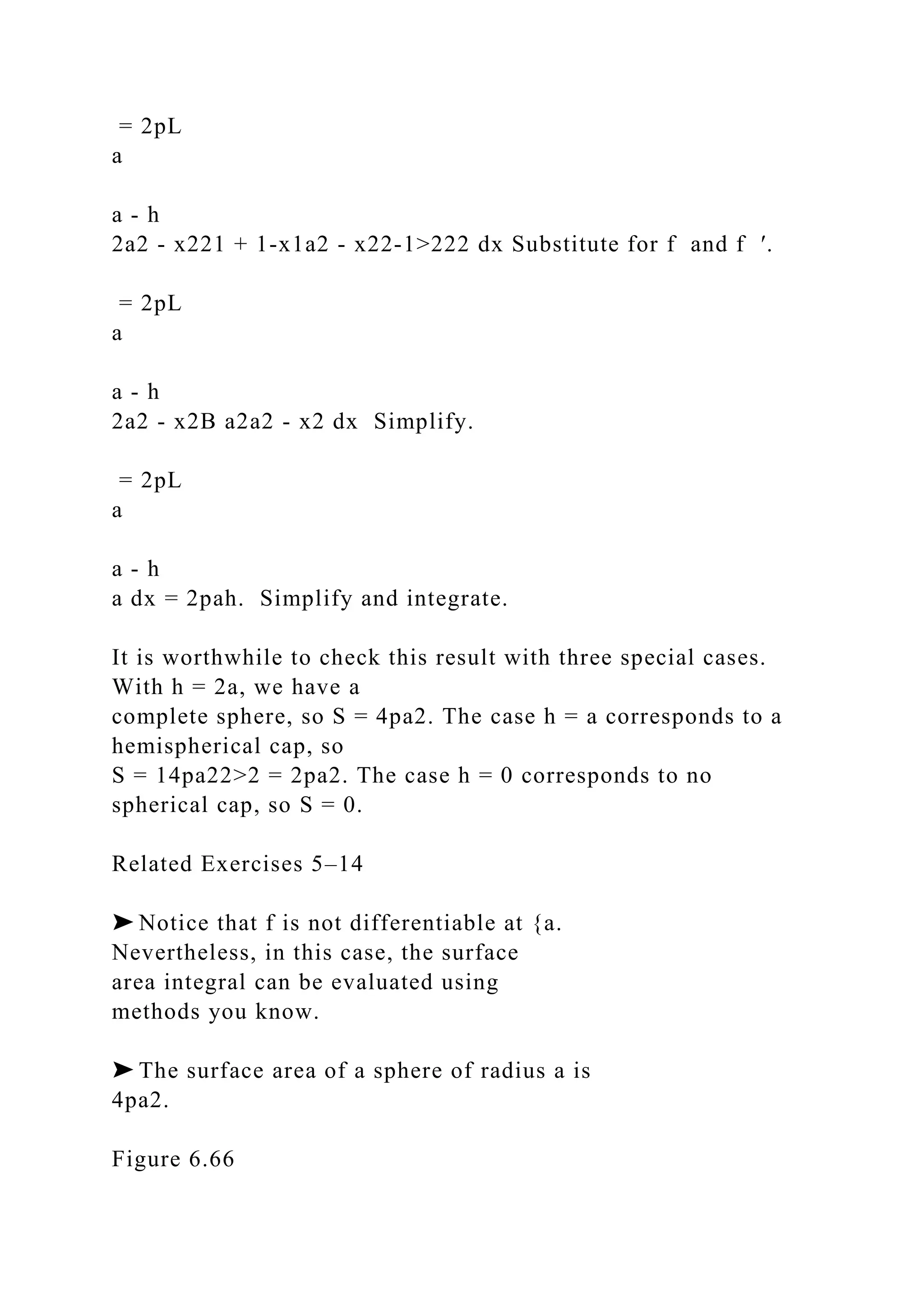
Exponential Decay Functions
Exponential decay is described by functions of the form y1t2 =
y0e-kt. The initial
value of y is y102 = y0, and the rate constant k 7 0 determines
the rate of decay.
Exponential decay is characterized by a constant relative decay
rate. The constant
half-life is T1>2 = ln 2k , with the same units as t.
M06_BRIG7345_02_SE_C06.9.indd 486 06/11/13 8:11 AM
Radiometric Dating A powerful method for estimating the age
of ancient objects (for
example, fossils, bones, meteorites, and cave paintings) relies
on the radioactive decay of
certain elements. A common version of radiometric dating uses
the carbon isotope [email protected],
which is present in all living matter. When a living organism
dies, it ceases to replace [email protected],
and the [email protected] that is present decays with a half-life
of about T1>2 = 5730 years. Comparing
the [email protected] in a living organism to the amount in a

dead sample provides an estimate of its age.
EXAMPLE 5 Radiometric dating Researchers determine that a
fossilized bone has
30% of the [email protected] of a live bone. Estimate the age of
the bone. Assume a half-life for [email protected]
of 5730 years.
SOLUTION The exponential decay function y1t2 = y0e-kt
represents the amount of
C-14 in the bone t years after its owner died. By the half-life
formula, T1>2 = 1ln 22>k.
Substituting T1>2 = 5730 yr, the rate constant is
k =
ln 2
T1>2 = ln 25730 yr ≈ 0.000121 yr-1.
Assume that the amount of [email protected] in a living bone is
y0. Over t years, the amount of
[email protected] in the fossilized bone decays to 30% of its
initial value, or 0.3y0. Using the decay
function, we have
0.3y0 = y0e-0.000121t.
Solving for t, the age of the bone (in years) is
t =
ln 0.3
-0.000121 ≈ 9950.
Pharmacokinetics Pharmacokinetics describes the processes by

which drugs are
assimilated by the body. The elimination of most drugs from
the body may be modeled by
an exponential decay function with a known half-life (alcohol is
a notable exception). The
simplest models assume that an entire drug dose is immediately
absorbed into the blood.
This assumption is a bit of an idealization; more refined
mathematical models account for
the absorption process.
EXAMPLE 6 Pharmacokinetics An exponential decay function
y1t2 = y0e-kt models
the amount of drug in the blood t hr after an initial dose of y0 =
100 mg is administered.
Assume the half-life of the drug is 16 hours.
a. Find the exponential decay function that governs the amount
of drug in the blood.
b. How much time is required for the drug to reach 1% of the
initial dose (1 mg)?
c. If a second 100-mg dose is given 12 hr after the first dose,
how much time is required
for the drug level to reach 1 mg?
SOLUTION
a. Knowing that the half-life is 16 hr, the rate constant is
k =
ln 2
T1>2 = ln 216 hr ≈ 0.0433 hr-1.
Therefore, the decay function is y1t2 = 100e-0.0433t.
b. The time required for the drug to reach 1 mg is the solution

of
100e-0.0433t = 1.
Solving for t, we have
t =
ln 0.01
-0.0433 hr-1
≈ 106 hr.
It takes more than 4 days for the drug to be reduced to 1% of
the initial dose.
➤ Half-lives of common drugs
Penicillin 1 hr
Amoxicillin 1 hr
Nicotine 2 hr
Morphine 3 hr
Tetracycline 9 hr
Digitalis 33 hr
Phenobarbitol 2–6 days
M06_BRIG7345_02_SE_C06.9.indd 487 21/10/13 11:37 AM
6.10 Hyperbolic Functions 491
6.10 Hyperbolic Functions
In this section, we introduce a new family of functions called
the hyperbolic functions,
which are closely related to both trigonometric functions and
exponential functions.

Hyperbolic functions find widespread use in applied problems
in fluid dynamics,
projectile motion, architecture, and electrical engineering, to
name just a few areas.
Hyperbolic functions are also important in the development of
many theoretical results in
mathematics.
Relationship Between Trigonometric and Hyperbolic Functions
The trigonometric functions defined in Chapter 1 are based on
relationships involving
a circle—for this reason, trigonometric functions are also
known as circular functions.
Specifically, cos t and sin t are equal to the x- and y-
coordinates, respectively, of the point
P1x, y2 on the unit circle that corresponds to an angle of t
radians (Figure 6.90). We can
also regard t as the length of the arc from 11, 02 to the point
P1x, y2.
Figure 6.90
x2 ! y2 " 1
1
y
x
Area " t/2
Three ways to interpret t :
t = angle in radians
t = arc length
t = 2 · (area of sector)
t

P(x, y) "
(cos t, sin t)
Arc
length " t
1
There is yet another way to interpret the number t, and it is this
third interpretation
that links the trigonometric and hyperbolic functions. Observe
that t is twice the area of
the circular sector in Figure 6.90. The functions cos t and sin t
are still defined as the
x- and y-coordinates of the point P, but now we associate P with
a sector whose area is
one-half of t.
The hyperbolic cosine and hyperbolic sine are defined in an
analogous fashion us-
ing the hyperbola x2 - y2 = 1 instead of the circle x2 + y2 = 1.
Consider the region
bounded by the x-axis, the right branch of the unit hyperbola x2
- y2 = 1, and a line seg-
ment from the origin to a point P1x, y2 on the hyperbola (Figure
6.91); let t equal twice the
area of this region.
The hyperbolic cosine of t, denoted cosh t, is the x-coordinate
of P and the hyperbolic
sine of t, denoted sinh t, is the y-coordinate of P. Expressing x
and y in terms of t leads to
the standard definitions of the hyperbolic functions. We
accomplish this task by writing t,
which is an area, as an integral that depends on the coordinates

of P. In Exercise 112, we
ask you to carry out the calculations to show that
x = cosh t =
et + e-t
2
and y = sinh t =
et - e-t
2
.
Everything that follows in this section is based on these two
definitions.
Definitions, Identities, and Graphs of the Hyperbolic Functions
Once the hyperbolic cosine and hyperbolic sine are defined, the
four remaining hyperbolic
functions follow in a manner analogous to the trigonometric
functions.
➤ Recall that the area of a circular sector of
radius r and angle u is A = 12 r2u. With
r = 1 and u = t, we have A = 12t, which
implies t = 2A.
Figure 6.91
1
x2 ! y2 " 1
y

P(x, y) "
(cosh t, sinh t)
x
t " twice the area
of hyperbolic sector
M06_BRIG7345_02_SE_C06.10.indd 491 21/10/13 11:30 AM
The hyperbolic functions satisfy many important identities.
Let’s begin with the fun-
damental identity for hyperbolic functions, which is analogous
to the familiar trigonomet-
ric identity cos2 x + sin2 x = 1:
cosh2 x - sinh2 x = 1.
This identity is verified by appealing to the definitions:
cosh2 x - sinh2 x = a ex + e-x
2
b2 - a ex - e-x
2
b2 Definition of cosh x and sinh x
=
e2x + 2 + e-2x - 1e2x - 2 + e-2x2
4

Expand and combine fractions.
=
4
4
= 1. Simplify.
EXAMPLE 1 Deriving hyperbolic identities
a. Use the fundamental identity cosh2 x - sinh2 x = 1 to prove
that 1 - tanh2 x = sech2 x.
b. Derive the identity sinh 2x = 2 sinh x cosh x.
SOLUTION
a. Dividing both sides of the fundamental identity cosh2 x -
sinh2 x = 1 by cosh2 x leads
to the desired result:
cosh2 x - sinh2 x = 1 Fundamental identity
cosh2 x
cosh2 x
- sinh
2 x
cosh2 x
=
1
cosh2 x
Divide both sides by cosh2 x.

(+)+* (+)+*
tanh2 x sech2 x
1 - tanh2 x = sech2 x. Identify functions.
b. Using the definition of the hyperbolic sine, we have
sinh 2x =
e2x - e-2x
2
Definition of sinh
=
1ex - e-x21ex + e-x2
2
Factor; difference of perfect squares
= 2 sinh x cosh x. Identify functions.
The identities in Example 1 are just two of many useful
hyperbolic identities, some of
which we list next.
➤ There is no universally accepted
pronunciation of the names of the
hyperbolic functions. In the United States,
cohsh x (long oh sound) and sinch x
are common choices for cosh x and sinh x.
The pronunciations tanch x, cotanch x,
seech x or sech x, and coseech x or
cosech x are used for the other functions.
International pronunciations vary as well.

➤ The fundamental identity for hyperbolic
functions can also be understood in
terms of the geometric definition of the
hyperbolic functions. Because the point
P1cosh t, sinh t2 is on the hyperbola
x2 - y2 = 1, the coordinates of P satisfy
the equation of the hyperbola, which leads
immediately to
cosh2 t - sinh2 t = 1.
DEFINITION Hyperbolic Functions
Hyperbolic cosine Hyperbolic sine
cosh x =
ex + e-x
2
sinh x =
ex - e-x
2
Hyperbolic tangent Hyperbolic cotangent
tanh x =
sinh x
cosh x
=
ex - e-x
ex + e-x coth x =
cosh x
sinh x

=
ex + e-x
ex - e-x
Hyperbolic secant Hyperbolic cosecant
sech x =
1
cosh x
=
2
ex + e-x csch x =
1
sinh x
=
2
ex - e-x
M06_BRIG7345_02_SE_C06.10.indd 492 21/10/13 11:30 AM
Graphs of the hyperbolic functions are relatively easy to
produce be-
cause they are based on the familiar graphs of ex and e-x.
Recall that
lim

xS ∞
e-x = 0 and that lim
xS- ∞
ex = 0. With these facts in mind, we see that
the graph of cosh x (Figure 6.92) approaches the graph of y =
1
2
ex as x S ∞
because cosh x =
ex + e-x
2
≈
ex
2
for large values of x. A similar argument
shows that as x S -∞ , cosh x approaches y = 1
2
e-x. Note also that cosh x
is an even function:
cosh1-x2 = e-x + e-1-x2
2
=
ex + e-x

2
= cosh x.
Finally, cosh 0 =
e0 + e0
2
= 1, so its y-intercept is 10, 12. The behavior of
sinh x, an odd function also shown in Figure 6.92, can be
explained in much
the same way.
Hyperbolic Identities
cosh2 x - sinh2 x = 1 cosh1-x2 = cosh x
1 - tanh2 x = sech2 x sinh1-x2 = -sinh x
coth2 x - 1 = csch2 x tanh1-x2 = - tanh x
cosh1x + y2 = cosh x cosh y + sinh x sinh y
sinh1x + y2 = sinh x cosh y + cosh x sinh y
cosh 2x = cosh2 x + sinh2 x sinh 2x = 2 sinh x cosh x
cosh2 x =
cosh 2x + 1
2
sinh2 x =
cosh 2x - 1
2
Figure 6.92
1
2
y

x!2 !1 1 2
2
!1
!2
y " !ex 1
2
y " !e!x
1
2
y " !!e!x
y " cosh x
domain (!#, #)
range [1, #)
(0, 1)
cosh x is an
even function
y " sinh x
domain (!#, #)
range (!#, #)
sinh x is an
odd function
Figure 6.93

!2 !1
2
1
!1
!2
(0, 1)
x1 2
y " tanh x
domain (!#, #)
range (!1, 1)
y " coth x
domain x ! 0
range |y| $ 1
!2 !1
y
2
1
!1
!2
y

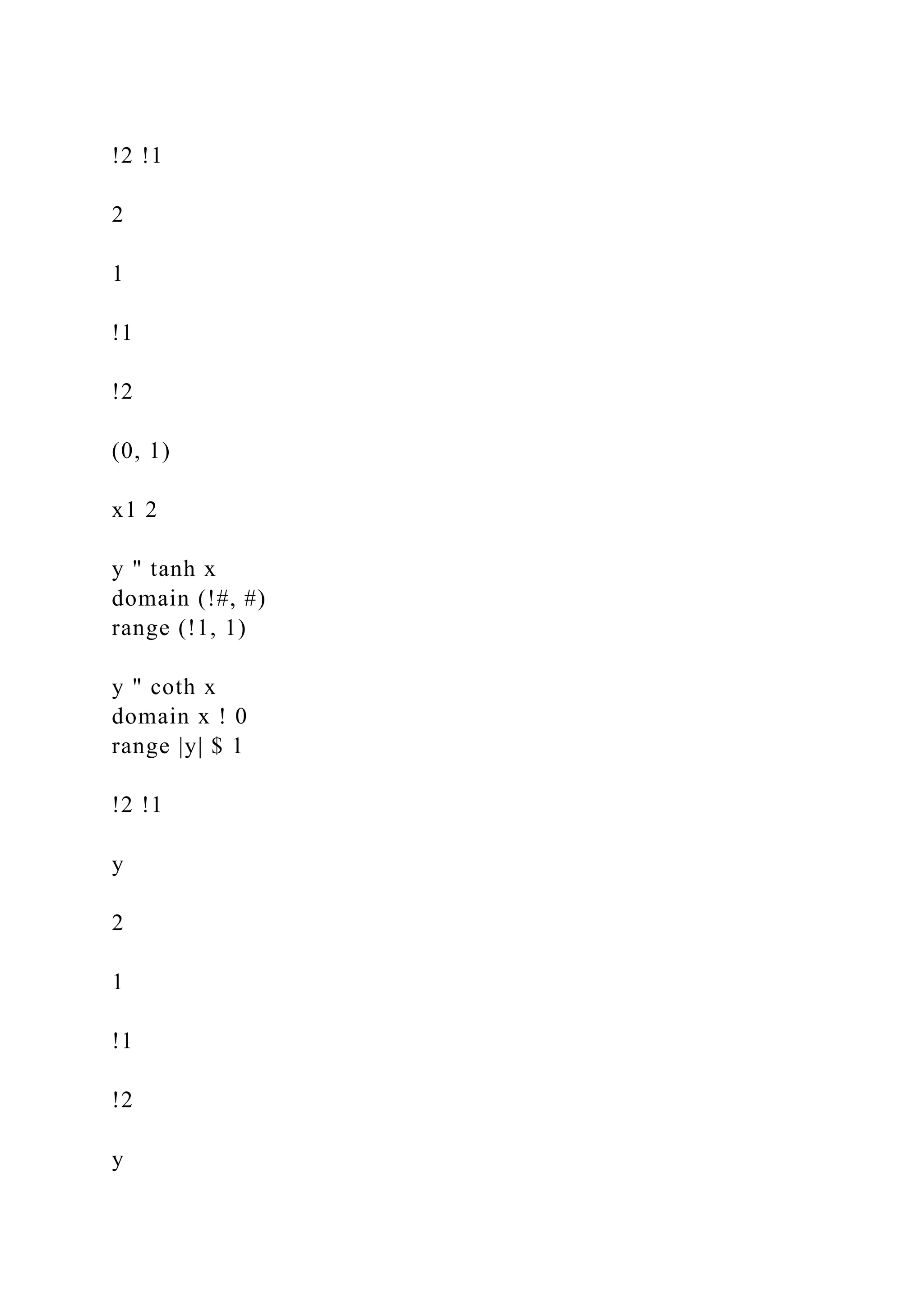
x1 2
y " sech x
domain (!#, #)
range (0, 1]
y " csch x
domain x ! 0
range y ! 0
QUICK CHECK 1 Use the definition of the hyperbolic sine to
show that sinh x is an odd
function.
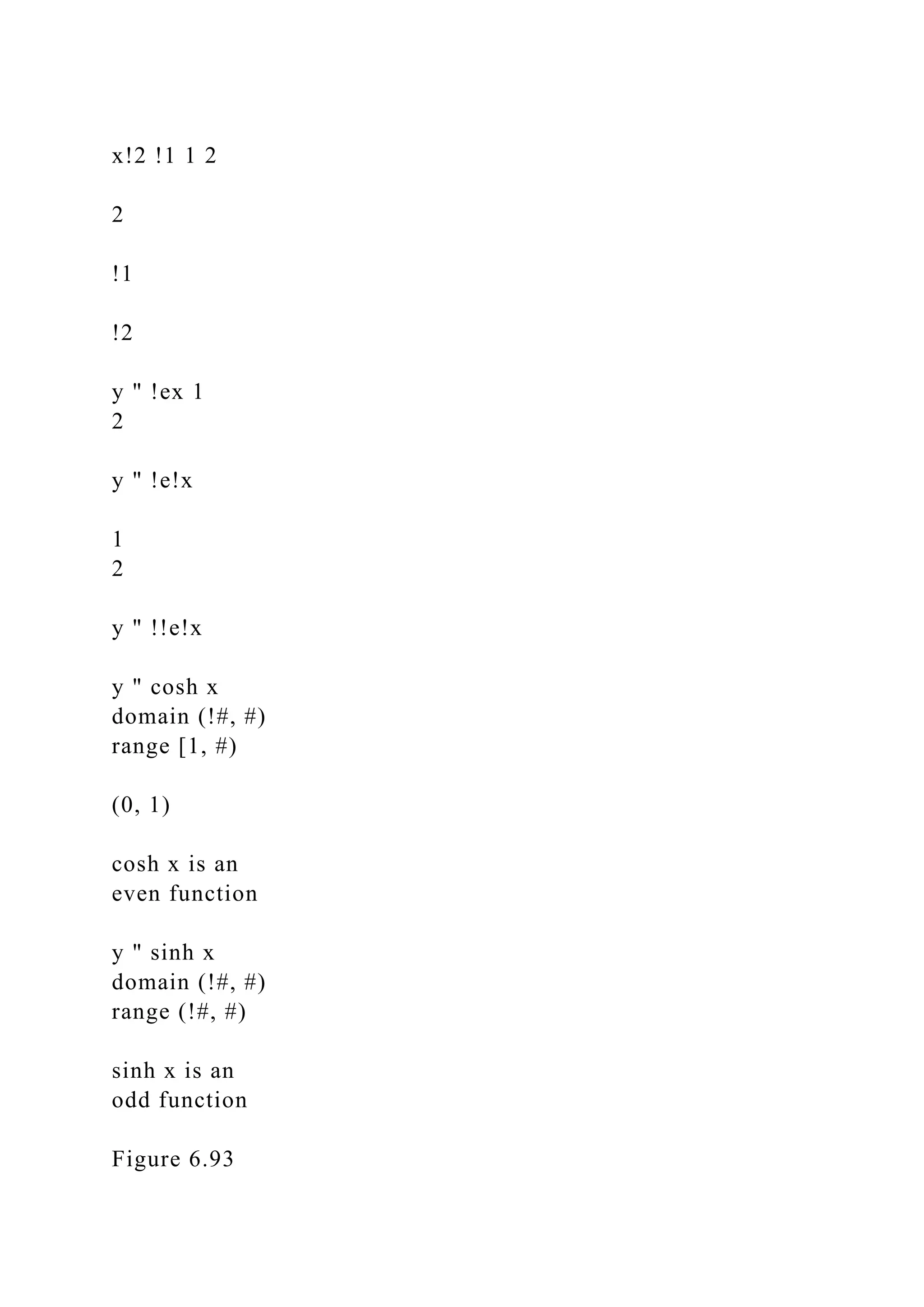
The graphs of the other four hyperbolic functions are shown in
Figure 6.93. As a con-
sequence of their definitions, we see that the domain of cosh x,
sinh x, tanh x, and sech x is 1- ∞ , ∞2, whereas the domain of
coth x and csch x is the set of all real numbers excluding 0.
QUICK CHECK 2 Explain why the graph of tanh x has the
horizontal asymptotes y = 1 and
y = -1.
M06_BRIG7345_02_SE_C06.10.indd 493 21/10/13 11:30 AM
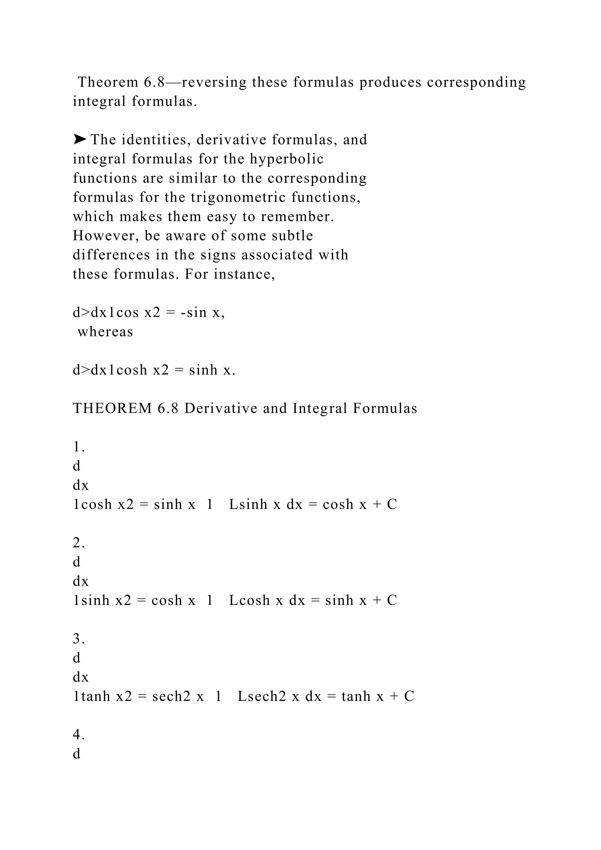
Derivatives and Integrals of Hyperbolic Functions
Because the hyperbolic functions are defined in terms of ex and
e-x, computing their
derivatives is straightforward. The derivatives of the hyperbolic
functions are given in

Theorem 6.8—reversing these formulas produces corresponding
integral formulas.
➤ The identities, derivative formulas, and
integral formulas for the hyperbolic
functions are similar to the corresponding
formulas for the trigonometric functions,
which makes them easy to remember.
However, be aware of some subtle
differences in the signs associated with
these formulas. For instance,
d>dx1cos x2 = -sin x,
whereas
d>dx1cosh x2 = sinh x.
THEOREM 6.8 Derivative and Integral Formulas
1.
d
dx
1cosh x2 = sinh x 1 Lsinh x dx = cosh x + C
2.
d
dx
1sinh x2 = cosh x 1 Lcosh x dx = sinh x + C
3.
d
dx
1tanh x2 = sech2 x 1 Lsech2 x dx = tanh x + C
4.
d

dx
1coth x2 = -csch2 x 1 Lcsch2 x dx = -coth x + C
5.
d
dx
1sech x2 = -sech x tanh x 1 Lsech x tanh x dx = -sech x + C
6.
d
dx
1csch x2 = -csch x coth x 1 Lcsch x coth x dx = -csch x + C
Proof: Using the definitions of cosh x and sinh x, we have
d
dx
1cosh x2 = d
dx
a ex + e-x
2
b = ex - e-x
2
= sinh x and
d
dx
1sinh x2 = d
dx

a ex - e-x
2
b = ex + e-x
2
= cosh x.
To prove formula (3), we begin with tanh x = sinh x>cosh x and
then apply the Quotient
Rule:
d
dx
1tanh x2 = d
dx
a sinh x
cosh x
b Definition of tanh x
=
cosh x1cosh x2 - sinh x1sinh x2
cosh2 x
Quotient Rule
=
1
cosh2 x
cosh2 x - sinh2 x = 1

= sech2 x. sech x = 1>cosh x
The proofs of the remaining derivative formulas are assigned in
Exercises 19–21. The
integral formulas are a direct consequence of their
corresponding derivative formulas.
EXAMPLE 2 Derivatives and integrals of hyperbolic functions
Evaluate the follow-
ing derivatives and integrals.
a.
d
dx
1sech 3x2 b. d2
dx2
1sech 3x2
c. L
csch2 1x1x dx d. L ln 30 sinh3 x cosh x dx
M06_BRIG7345_02_SE_C06.10.indd 494 21/10/13 11:30 AM
SOLUTION
a. Combining formula (5) of Theorem 6.8 with the Chain Rule
gives
d

dx
1sech 3x2 = -3 sech 3x tanh 3x.
b. Applying the Product Rule and Chain Rule to the result of
part (a), we have
d2
dx2
1sech 3x2 = d
dx
1-3 sech 3x tanh 3x2
=
d
dx
1-3 sech 3x2 # tanh 3x + 1-3 sech 3x2 # d
dx
1tanh 3x2 Product Rule
v u
9 sech 3x tanh 3x 3 sech2 3x
= 9 sech 3x tanh2 3x - 9 sech3 3x Chain Rule
= 9 sech 3x1tanh2 3x - sech2 3x2. Simplify.
c. The integrand suggests the substitution u = 1x:
L
csch2 1x1x dx = 2Lcsch2 u du Let u = 1x ; du = 121x dx.
= -2 coth u + C Formula (4), Theorem 6.8
= -2 coth 1x + C. u = 1x

d. The derivative formula d>dx1sinh x2 = cosh x suggests the
substitution u = sinh x:
L
ln 3
0
sinh3 x cosh x dx = L
4>3
0
u3 du. Let u = sinh x; du = cosh x dx.
The new limits of integration are determined by the calculations
x = 0 1 u = sinh 0 = 0 and
x = ln 3 1 u = sinh1ln 32 = eln 3 - e-ln 3
2
=
3 - 1>3
2
=
4
3
.
We now evaluate the integral in the variable u:
L

4>3
0
u3 du =
1
4
u4 ` 4>3
0
=
1
4
aa 4
3
b4 - 04b = 64
81
.
QUICK CHECK 3 Find both the derivative and indefinite
integral of f 1x2 = 4 cosh 2x.
Theorem 6.9 presents integral formulas for the four hyperbolic
functions not covered
in Theorem 6.8.
THEOREM 6.9 Integrals of Hyperbolic Functions
1. L tanh x dx = ln cosh x + C 2. Lcoth x dx = ln ! sinh x ! + C
3. Lsech x dx = tan-11sinh x2 + C 4. Lcsch x dx = ln !
tanh1x>22 ! + C

M06_BRIG7345_02_SE_C06.10.indd 495 21/10/13 11:31 AM
Proof: Formula (1) is derived by first writing tanh x in terms of
sinh x and cosh x:
L tanh x dx = L
sinh x
cosh x
dx Definition of tanh x
= L
1
u
du Let u = cosh x; du = sinh x dx.
= ln ! u ! + C Evaluate integral.
= ln cosh x + C. u = cosh x 7 0
Formula (2) is derived in a similar fashion (Exercise 44). The
more challenging proofs
of formulas (3) and (4) are considered in Exercises 107 and 108.
EXAMPLE 3 Integrals involving hyperbolic functions
Determine the indefinite
integral 1x coth 1x22 dx.
SOLUTION The integrand suggests the substitution u = x2:
Lx coth x2 dx =
1

2 Lcoth u du. Let u = x2; du = 2x dx.
=
1
2
ln ! sinh u ! + C Evaluate integral; use Theorem 6.9.
=
1
2
ln1sinh x22 + C. u = x2; sinh x2 Ú 0
QUICK CHECK 4 Determine the indefinite integral 1csch 2x
dx.
Inverse Hyperbolic Functions
At present, we don’t have the tools for evaluating an integral
such as L
dx2x2 + 4.
By studying inverse hyperbolic functions, we can discover new
integration formulas.
Inverse hyperbolic functions are also useful for solving
equations involving hyperbolic
functions.
Figures 6.92 and 6.93 show that the functions sinh x, tanh x,
coth x, and csch x are all
one-to-one on their respective domains. This observation
implies that each of these func-
tions has a well-defined inverse. However, the function y = cosh
x is not one-to-one on 1- ∞ , ∞2, so its inverse, denoted y =
cosh-1 x, exists only if we restrict the domain of

cosh x. Specifically, when y = cosh x is restricted to the interval
30, ∞2, it is one-to-one,
and its inverse is defined as follows:
y = cosh-1 x if and only if x = cosh y, for x Ú 1 and 0 … y 6 ∞
.
Figure 6.94a shows the graph of y = cosh-1 x, obtained by
reflecting the graph of
y = cosh x on 30, ∞2 over the line y = x. The definitions and
graphs of the other five
inverse hyperbolic functions are also shown in Figure 6.94.
Notice that the domain of
y = sech x (Figure 6.94d) must be restricted to 30, ∞2 to ensure
the existence of its
inverse.
Because hyperbolic functions are defined in terms of
exponential functions, we can
find explicit formulas for their inverses in terms of logarithms.
For example, let’s start
with the definition of the inverse hyperbolic sine. For all real x
and y, we have
y = sinh-1 x 3 x = sinh y.
M06_BRIG7345_02_SE_C06.10.indd 496 21/10/13 11:31 AM
Following the procedure outlined in Section 1.3, we solve
x = sinh y =
ey - e-y

2
for y to give a formula for sinh-1 x:
x =
ey - e-y
2
1 ey - 2x - e-y = 0 Rearrange equation.
1 1ey22 - 2xey - 1 = 0. Multiply by ey.
At this stage, we recognize a quadratic equation in ey and solve
for ey using the quadratic
formula, with a = 1, b = -2x, and c = -1:
ey =
2x { 24x2 + 4
2
= x { 2x2 + 1 = x + 2x2 + 1.
choose positive root
Because ey 7 0 and 2x2 + 1 7 x, the positive root must be
chosen. We now solve for y
by taking the natural logarithm of both sides:
ey = x + 2x2 + 1 1 y = ln1x + 2x2 + 12.
Therefore, the formula we seek is sinh-1 x = ln1x + 2x2 + 12.
A similar procedure can be carried out for the other inverse
hyperbolic functions
(Exercise 110). Theorem 6.10 lists the results of these
calculations.

y ! cosh"1 x
y ! cosh x
y ! cosh"1 x ⇔x ! cosh y
for x # 1 and 0 $ y % &
(a)
y
x
2
1
1 2
y ! sinh x
y ! sinh"1 x
y ! sinh"1 x ⇔x ! sinh y
for "# $ x $ # and "# $ y $ #
(b)
y
x21"1"2
"2
"1

1
2
y ! tanh"1 x ⇔x ! tanh y
for "1 # x # 1 and "$ # y # $
(c)
y ! tanh x
y ! tanh"1 x
y
x321
"1
1
2
3
"2
"3
"1"2"3
Figure 6.94
y ! sech"1 x
y ! sech x
y ! sech"1 x ⇔x ! sech y

for 0 # x $ 1 and 0 $ y # %
(d)
y
x321
3
2
1
y ! csch"1 x
y ! csch x
y ! csch"1 x ⇔x ! csch y
for x ! 0 and y ! 0
(e)
y
x21"1"2
"2
"1
1
2
y ! coth"1 x ⇔x ! coth y

for |x| # 1 and y ! 0
( f )
y
x21"1"2
"2
"1
1
2
y ! coth"1 x
y ! coth x
v
M06_BRIG7345_02_SE_C06.10.indd 497 21/10/13 11:31 AM
Notice that the formulas in Theorem 6.10 for the inverse
hyperbolic secant, cosecant,
and cotangent are given in terms of the inverses of their
corresponding reciprocal func-
tions. Justification for these formulas follows from the
definitions of the inverse functions.
For example, from the definition of csch-1 x, we have

y = csch-1 x 3 x = csch y 3 1>x = sinh y.
Applying the inverse hyperbolic sine to both sides of 1>x = sinh
y yields
sinh-111>x2 = sinh-11sinh y2 or y = csch-1 x = sinh-111>x2.
u
y
Similar derivations yield the other two formulas.
EXAMPLE 4 Points of intersection Find the points at which the
curves y = cosh x
and y = 53 intersect (Figure 6.95).
SOLUTION The x-coordinates of the points of intersection
satisfy the equation
cosh x = 53, which is solved by applying cosh-1 to both sides of
the equation. However,
evaluating cosh-11cosh x2 requires care—in Exercise 105, you
are asked to show that
cosh-11cosh x2 = ! x ! . With this fact, the points of intersection
can be found:
cosh x = 53 Set equations equal to one another.
cosh-11cosh x2 = cosh-1 53 Apply cosh-1 to both sides.
! x ! = ln153 + 215322 - 12 Simplify; use Theorem 6.10.
x = { ln 3. Simplify.
The points of intersection lie on the line y = 53, so the points
are 1- ln 3, 532 and 1ln 3, 532.
Derivatives of the Inverse Hyperbolic Functions
and Related Integral Formulas

The derivatives of the inverse hyperbolic functions can be
computed directly from the
logarithmic formulas given in Theorem 6.10. However, it is
more efficient to use the
definitions in Figure 6.94.
Recall that the inverse hyperbolic sine is defined by
y = sinh-1 x 3 x = sinh y.
We differentiate both sides of x = sinh y with respect to x and
solve for dy>dx:
x = sinh y y = sinh-1 x 3 x = sinh y
1 = 1cosh y2 dy
dx
Use implicit differentiation.
dy
dx
=
1
cosh y
Solve for dy>dx.
dy
dx
=
1

{2sinh2 y + 1 cosh2 y - sinh2 y = 1
dy
dx
=
12x2 + 1. x = sinh y
Figure 6.95
x1
y
2
1 y ! cosh x
"1
5y ! 3
THEOREM 6.10 Inverses of the Hyperbolic Functions
Expressed as Logarithms
cosh-1 x = ln 1x + 2x2 - 12 1x Ú 12 sech-1 x = cosh-1 1
x
10 6 x … 12
sinh-1 x = ln 1x + 2x2 + 12 csch-1 x = sinh-1 1
x
1x ≠ 02

tanh-1 x =
1
2
ln a 1 + x
1 - x b 1 ! x ! 6 12 coth-1 x = tanh-1 1x 1 ! x ! 7 12
➤ Most calculators allow for the direct
evaluation of the hyperbolic sine, cosine,
and tangent, along with their inverses, but
are not programmed to evaluate sech-1 x,
csch-1 x, and coth-1 x. The formulas in
Theorem 6.10 are useful for evaluating
these functions on a calculator.
QUICK CHECK 5 Use the results of
Example 4 to write an integral for
the area of the region bounded by
y = cosh x and y = 53 (Figure 6.95)
and then evaluate the integral.
M06_BRIG7345_02_SE_C06.10.indd 498 21/10/13 11:31 AM
The restrictions associated with the formulas in Theorem 6.11
are a direct conse-
quence of the domains of the inverse functions (Figure 6.94).
Note that the derivative of
both tanh-1 x and coth-1 x is 1>11 - x22, although this result is
valid on different domains 1 ! x ! 6 1 for tanh-1 x and ! x ! 7 1
for coth-1 x2. These facts have a bearing on formula
(3) in the next theorem, which is a reversal of the derivative
formulas in Theorem 6.11.

Here we list integral results, where a is a positive constant; each
formula can be verified
by differentiation.
THEOREM 6.11 Derivatives of the Inverse Hyperbolic
Functions
d
dx
1cosh-1 x2 = 12x2 - 1 1x 7 12 ddx 1sinh-1x2 = 12x2 + 1
d
dx
1tanh-1 x2 = 1
1 - x2
1 ! x ! 6 12 d
dx
1coth-1 x2 = 1
1 - x2
1 ! x ! 7 12
d
dx
1sech-1 x2 = - 1
x21 - x2 10 6 x 6 12 ddx 1csch-1 x2 = - 1! x ! 21 + x2 1x ≠ 02
THEOREM 6.12 Integral Formulas
1. L

dx2x2 - a2 = cosh-1 xa + C, for x 7 a
2. L
dx2x2 + a2 = sinh-1 xa + C, for all x
3. L
dx
a2 - x2
= µ 1a tanh-1 xa + C, for ! x ! 6 a
1
a
coth-1
x
a
+ C, for ! x ! 7 a
4. L
dx
x2a2 - x2 = - 1a sech-1 xa + C, for 0 6 x 6 a
5. L
dx
x2a2 + x2 = - 1a csch-1 ! x !a + C, for x ≠ 0
EXAMPLE 5 Derivatives of inverse hyperbolic functions
Compute dy>dx for each
function.
a. y = tanh-1 3x b. y = x2 sinh-1 x
SOLUTION

a. Using the Chain Rule, we have
dy
dx
=
d
dx
1tanh-1 3x2 = 1
1 - 13x22 # 3 = 31 - 9x2.
b.
dy
dx
= 2x sinh-1 x + x2 # 12x2 + 1 Product Rule; Theorem 6.11
= x a22x2 + 1 # sinh-1 x + x2x2 + 1 b Simplify.
➤ The integrals in Theorem 6.12 appear
again in Chapter 7 in terms of logarithms
and with fewer restrictions on the
variable of integration.
➤ The function 3>11 - 9x22 in the
solution to Example 5a is defined for all
x ≠ {1>3. However, the derivative
formula dy>dx = 3>11 - 9x22 is
valid only on -1>3 6 x 6 1>3
because tanh-1 3x is defined only
on -1>3 6 x 6 1>3. The result of
computing d>dx1coth-1 3x2 is the same,

but valid on 1- ∞ , -1>32 ∪ 11>3, ∞2.
In the last step, the positive root is chosen because cosh y 7 0
for all y.
The derivatives of the other inverse hyperbolic functions, listed
in Theorem 6.11, are
derived in a similar way (Exercise 106).
M06_BRIG7345_02_SE_C06.10.indd 499 21/10/13 11:31 AM
EXAMPLE 6 Integral computations
a. Compute the area of the region bounded by y = 1>2x2 + 16
over the interval 30, 34.
b. Evaluate L
25
9
dx1x14 - x2.
SOLUTION
a. The region in question is shown in Figure 6.96, and its area is
given by
L
3
0

dx2x2 + 16. Using formula (2) in Theorem 6.12 with a = 4, we
have
L
3
0
dx2x2 + 16 = sinh-1 x4 ` 30 Theorem 6.12
= sinh-1
3
4
- sinh-1 0 Evaluate.
= sinh-1
3
4
. sinh-10 = 0
A calculator gives an approximate result of sinh-113>42 ≈
0.693. The exact result
can be written in terms of logarithms using Theorem 6.10:
sinh-113>42 = ln13>4 + 213>422 + 12 = ln 2.
b. The integral doesn’t match any of the formulas in Theorem
6.12, so we use the substi-
tution u = 1x:
L
25
9

dx1x14 - x2 = 2L53 du4 - u2. Let u = 1x; du = dx21x .
The new integral now matches formula (3), with a = 2. We
conclude that
2L
5
3
du
4 - u2
= 2 # 1
2
coth-1
u
2
` 5
3
L
dx
a2 - x2
=
1
a
coth-1
x
a

+ C
= coth-1
5
2
- coth-1 3
2
. Evaluate.
The antiderivative involving coth-1 x was chosen because the
interval of integration 13 … u … 52 satisfies " u " 7 a = 2.
Theorem 6.10 is used to express the result in
numerical form in case your calculator cannot evaluate coth-1 x:
coth-1
5
2
- coth-1 3
2
= tanh-1
2
5
- tanh-1 2
3
≈ -0.381.
QUICK CHECK 6 Evaluate L
1

0
du
4 - u2
.
Applications of Hyperbolic Functions
This section concludes with a brief look at two applied
problems associated with hyper-
bolic functions. Additional applications are presented in the
exercises.
The Catenary When a free-hanging rope or flexible cable
supporting only its own
weight is attached to two points of equal height, it takes the
shape of a curve known as
a catenary. You can see catenaries in telephone wires, ropes
strung across chasms for
Tyrolean traverses (Example 7), and spider webs.
The equation for a general catenary is y = a cosh1x>a2, where a
≠ 0 is a real num-
ber. When a 6 0, the curve is called an inverted catenary,
sometimes used in the design
of arches. Figure 6.97 illustrates catenaries for several values of
a.
Figure 6.96
x
1
x2 ! 16

y "
0.25
y
321#1
y ! acosh(x/a)
for several values
of a " 0
When a # 0,
inverted catenaries
result (reflections
across the x-axis)
a ! 0.5
a ! 1.0
a ! 2.0
a ! 1.5
a ! 3.0
x41 2 3
y
5
4
3

2
1
$1$2$3$4
Figure 6.97
M06_BRIG7345_02_SE_C06.10.indd 500 21/10/13 11:31 AM
EXAMPLE 7 Length of a catenary A climber anchors a rope at
two points of equal
height, separated by a distance of 100 ft, in order to perform a
Tyrolean traverse. The
rope follows the catenary f 1x2 = 200 cosh1x>2002 over the
interval 3-50, 504
(Figure 6.98). Find the length of the rope between the two
anchor points.
➤ A Tyrolean traverse is used to pass over
difficult terrain, such as a chasm between
two cliffs or a raging river. A rope is
strung between two anchor points, the
climber clips onto the rope and then
traverses the gap by pulling on the rope. y
100
200
x50!50

y " 200 cosh (x /200)
Figure 6.98
SOLUTION Recall from Section 6.5 that the arc length of the
curve y = f 1x2 over the
interval 3a, b4 is L = Lba 21 + f ′1x22 dx. Also note that
f ′1x2 = 200 sinh a x
200
b # 1
200
= sinh
x
200
.
Therefore, the length of the rope is
L = L
50
-50 B1 + sinh2a x200 b dx Arc length formula
= 2L
50
0 B1 + sinh2a x200 b dx Use symmetry.
= 400L
1>4
0

21 + sinh2 u du Let u = x
200
.
= 400L
1>4
0
cosh u du 1 + sinh2 u = cosh2 u
= 400 sinh u ` 1>4
0
Evaluate integral.
= 400asinh 1
4
- sinh 0b Simplify.
≈ 101 ft. Evaluate. Related Exercises 65–68
Velocity of a Wave To describe the characteristics of a
traveling wave, research-
ers formulate a wave equation that reflects the known (or
hypothesized) properties of
the wave and that often takes the form of a differential equation
(Section 7.9). Solving a
wave equation produces additional information about the wave,
and it turns out that hyper-
bolic functions may arise naturally in this context.
EXAMPLE 8 Velocity of an ocean wave The velocity v (in
meters/second) of an ideal-
ized surface wave traveling on the ocean is modeled by the

equation
v = B gl2p tanha 2pdl b ,
➤ Using the principles of vector analysis
introduced in Chapter 11, the tension in
the rope and the forces acting upon the
anchors in Example 7 can be computed.
This is crucial information for anyone
setting up a Tyrolean traverse; the sag
angle (Exercise 68) figures into these
calculations. Similar calculations are
important for catenary lifelines used in
construction and for rigging camera shots
in Hollywood movies.
M06_BRIG7345_02_SE_C06.10.indd 501 21/10/13 11:31 AM
5. Express sinh-1 x in terms of logarithms.
6. What is the domain of sech-1 x? How is sech-1 x defined in
terms
of the inverse hyperbolic cosine?
7. A calculator has a built-in sinh-1 x function, but no csch-1 x
func-
tion. How do you evaluate csch-1 5 on such a calculator?
8. On what interval is the formula d>dx1tanh-1 x2 = 1>1x2 - 12
valid?
where g = 9.8 m>s2 is the acceleration due to gravity, l is the

wavelength measured in
meters from crest to crest, and d is the depth of the undisturbed
water, also measured in
meters (Figure 6.99).
a. A sea kayaker observes several waves that pass beneath her
kayak, and she estimates
that l = 12 m and v = 4 m>s. How deep is the water in which she
is kayaking?
b. The deep-water equation for wave velocity is v = A gl2p,
which is an approximation
to the velocity formula given above. Waves are said to be in
deep water if the depth-
to-wavelength ratio d>l is greater than 1
2
. Explain why v = A gl2p is a good approxi-
mation when d>l 7 1
2
.
SOLUTION
a. We substitute l = 12 and v = 4 into the velocity equation and
solve for d.
4 = B g # 122p tanha 2pd12 b 1 16 = 6gp tanhapd6 b Square
both sides.
1 8p
3g
= tanhapd

6
b Multiply by p
6g
.
In order to extract d from the argument of tanh, we apply tanh-1
to both sides of the
equation and then use the property tanh-11tanh x2 = x, for all x.
tanh-1a 8p
3g
b = tanh-1 a tanhapd
6
b b Apply tanh-1 to both sides.
tanh-1a 8p
29.4
b = pd
6
Simplify; 3g = 29.4.
d =
6
p
tanh-1a 8p
29.4
b ≈ 2.4 m Solve for d.
Therefore, the kayaker is in water that is about 2.4 m deep.
b. Recall that y = tanh x is an increasing function 1dy>dx =

sech2 x 7 02 whose values
approach 1 as x S ∞ . Also notice that when d
l
=
1
2
, tanha 2pd
l
b = tanh p ≈ 0.996,
which is nearly equal to 1. These facts imply that whenever
d
l
7 1
2
, we can replace
tanha 2pd
l
b with 1 in the velocity formula, resulting in the deep-water
velocity
function v = A gl2p.
➤ In fluid dynamics, water depth is often
discussed in terms of the depth-to-
wavelength ratio d>l, not the actual
depth of the water. Three classifications

are generally used:
shallow water: d>l 6 0.05
intermediate depth: 0.05 6 d>l 6 0.5
deep water: d>l 7 0.5
λ
d
Figure 6.99
x31 2
y
!1!2!3
tanh x ! 1 as x ! "
y # tanh x
!1
1
QUICK CHECK 7 Explain why longer
waves travel faster than shorter waves
in deep water.
Review Questions
1. State the definition of the hyperbolic cosine and hyperbolic
sine
functions.

2. Sketch the graphs of y = cosh x, y = sinh x, and y = tanh x
(include asymptotes), and state whether each function is even,
odd, or neither.
3. What is the fundamental identity for hyperbolic functions?
4. How are the derivative formulas for the hyperbolic functions
and
the trigonometric functions alike? How are they different?
M06_BRIG7345_02_SE_C06.10.indd 502 21/10/13 11:31 AM

Amazon.comThe three main activities that e.docx

More Related Content

Similar to Amazon.comThe three main activities that e.docx

More from nettletondevon

Recently uploaded

Amazon.comThe three main activities that e.docx