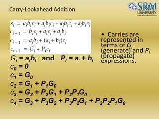
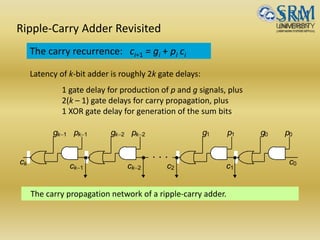
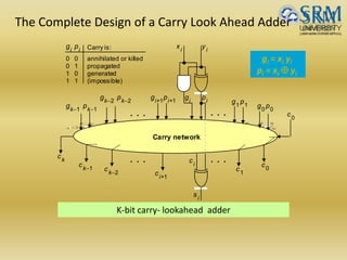
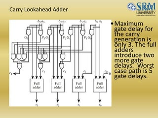
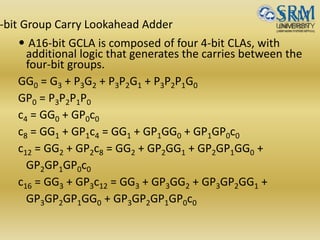
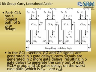
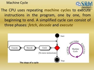
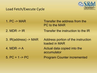
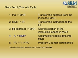
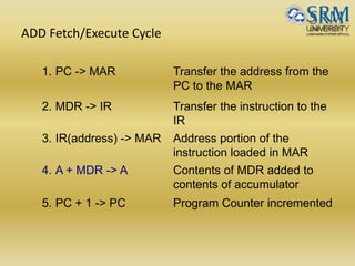
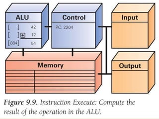
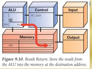
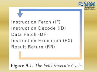
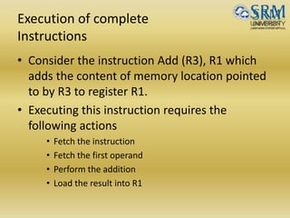
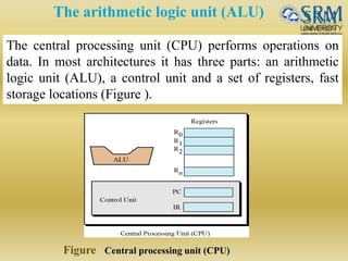
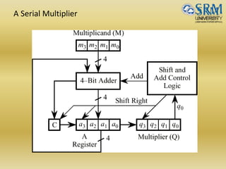
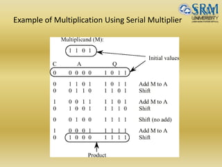
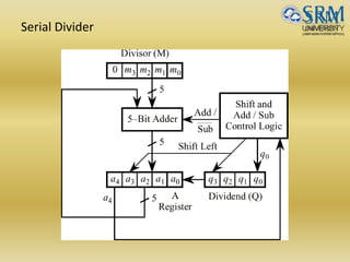
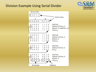
The document discusses various aspects of central processing unit (CPU) architecture and arithmetic operations. It covers the main components of a CPU - the arithmetic logic unit (ALU), control unit, and registers. It then describes different data representation methods including fixed-point and floating-point numbers. Various arithmetic operations for both types of numbers such as addition, subtraction, multiplication, and division are explained. Different adder designs like ripple-carry adder and carry lookahead adder are also summarized.
![Digit Sets and Encodings
Conventional and unconventional digit sets
Decimal digits in [0, 9]; 4-bit BCD, 8-bit ASCII
Hexadecimal, or hex for short: digits 0-9 & a-f
Conventional digit set for radix r is [0, r – 1]
Conventional binary digit set in [0, 1]](https://image.slidesharecdn.com/unitii-170523232217/85/BOOTH-ALGO-DIVISION-RESTORING-_-NON-RESTORING-etc-etc-4-320.jpg)
![Fixed-Point Numbers
Positional representation: k whole and l fractional digits
Value of a number: x = (xk–1xk–2 . . .x1x0 .x–1x–2 . . . x–l )r = S xi r i
For example:
2.375 = (10.011)two = (121) + (020) + (02-1) + (12-2) + (12-3)
Numbers in the range [0, rk – ulp] representable, where ulp = r–l
Fixed-point arithmetic same as integer arithmetic
(radix point implied, not explicit)
Two’s complement properties (including sign change) hold here as well:
(01.011)2’s-compl = (–021) + (120) + (02–1) + (12–2) + (12–3) = +1.375
(11.011)2’s-compl = (–121) + (120) + (02–1) + (12–2) + (12–3) = –0.625](https://image.slidesharecdn.com/unitii-170523232217/85/BOOTH-ALGO-DIVISION-RESTORING-_-NON-RESTORING-etc-etc-7-320.jpg)

![Unsigned Binary Integers
Schematic representation of 4-bit code for integers in [0,
15].
0000
00011111
00101110
00111101
01001100
1000
01011011
01101010
01111001
0
1
2
3
4
5
6
7
15
11
14
13
12
8
9
10
Inside: Natural number
Outside: 4-bit encoding
0
1
2
3
15
4
5
6
789
Turn x notches
counterclockwise
to add x
Turn y notches
clockwise
to subtract y
11
14
13
12
10](https://image.slidesharecdn.com/unitii-170523232217/85/BOOTH-ALGO-DIVISION-RESTORING-_-NON-RESTORING-etc-etc-9-320.jpg)

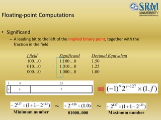
![Floating-point Computations
• Representation: (fraction, exponent) Has three fields:
sign, significant digits and exponent
eg.111101.100110 1.11101100110*25
• Value representation = +/- M*2 E’-127
In case of a 32 bit number 1 bit represents sign
8 bits represents exponent E’=E +127(bias) [ excess 127
format]
23 bits represents Mantissa](https://image.slidesharecdn.com/unitii-170523232217/85/BOOTH-ALGO-DIVISION-RESTORING-_-NON-RESTORING-etc-etc-19-320.jpg)
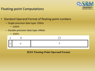
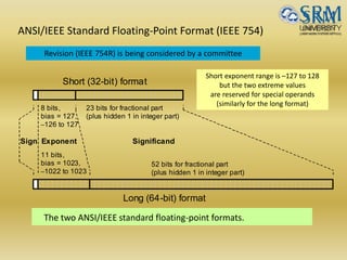
![Short and Long IEEE 754 Formats: Features
Table Some features of ANSI/IEEE standard floating-point formats
Feature Single/Short Double/Long
Word width in bits 32 64
Significand in bits 23 + 1 hidden 52 + 1 hidden
Significand range [1, 2 – 2–23] [1, 2 – 2–52]
Exponent bits 8 11
Exponent bias 127 1023
Zero (±0) e + bias = 0, f = 0 e + bias = 0, f = 0
Denormal e + bias = 0, f ≠ 0
represents ±0.f 2–126
e + bias = 0, f ≠ 0
represents ±0.f 2–1022
Infinity (∞) e + bias = 255, f = 0 e + bias = 2047, f = 0
Not-a-number (NaN) e + bias = 255, f ≠ 0 e + bias = 2047, f ≠ 0
Ordinary number e + bias [1, 254]
e [–126, 127]
represents 1.f 2e
e + bias [1, 2046]
e [–1022, 1023]
represents 1.f 2e
min 2–126 1.2 10–38 2–1022 2.2 10–308
max 2128 3.4 1038 21024 1.8 10308](https://image.slidesharecdn.com/unitii-170523232217/85/BOOTH-ALGO-DIVISION-RESTORING-_-NON-RESTORING-etc-etc-25-320.jpg)