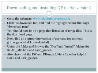
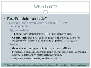
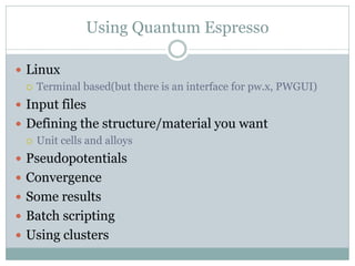
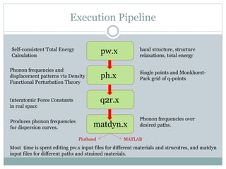
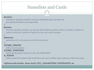
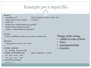
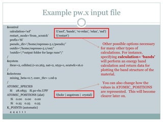
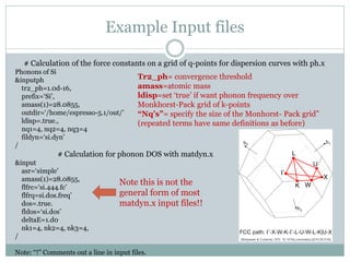
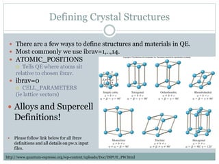
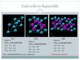
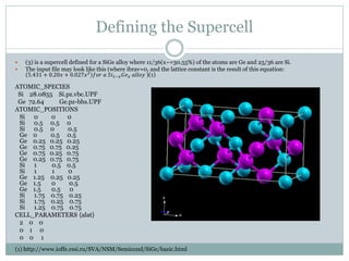
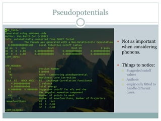
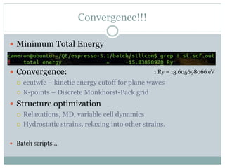
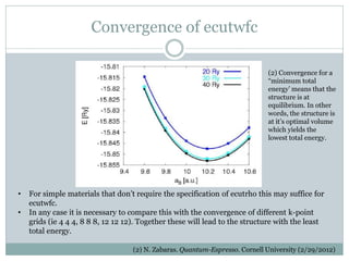
Quantum Espresso is a suite of open-source computer codes for electronic structure calculations and materials modeling based on density functional theory and plane waves. It can be used to calculate material properties including ground-state energy, atomic forces, stresses, molecular dynamics, and more. The document provides an introduction and overview of Quantum Espresso, including examples of input files for defining crystal structures, pseudopotentials, k-points, and performing calculations of total energy and phonon frequencies. Convergence of key parameters like the plane wave cutoff energy and k-point sampling is also discussed.

![Effects of Strain in QE
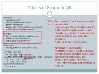
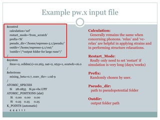
&control
calculation=‘scf’
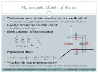
restart_mode=‘from_scratch’
prefix=‘Strained_Si’
pseudo_dir=‘/home/espresso-5.1/pseudo/’
outdir=‘/home/espresso-5.1/out/’
/
&system
ibrav=10, A=5.646.B=5.646,C=5.234,
cosAB=0, cosBC=0, cosAC=0,
nat=2, ntyp=1, ecutwfc=16.0
/
&electrons
mixing_beta=0.7, conv_thr= 1.0d-9
/
ATOMIC_SPECIES
Si 28.0855 Si.pz-vbc.UPF
ATOMIC_POSITIONS {crystal | alat | bohr | angstrom}
Si 0.00 0.00 0.00
Si 0.25 0.25 0.25
K_POINTS {automatic}
4 4 4 1 1 1
- BZ is morphed due to the
strain. (Be careful of what
kind of effect this is.)
[−
2𝜋
𝑎
,
2𝜋
𝑎
]](https://image.slidesharecdn.com/bd0e802e-6d10-4aa7-8e7f-2582dda4f32a-160324100124/85/Quantum-Espresso_10_8_14-21-320.jpg)