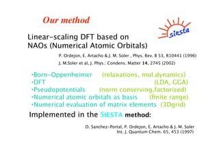
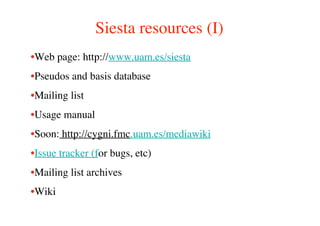
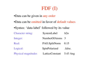
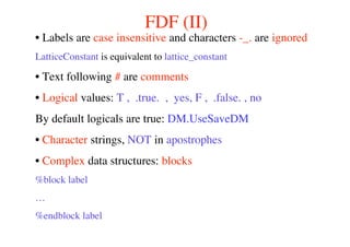
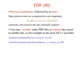
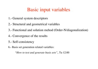
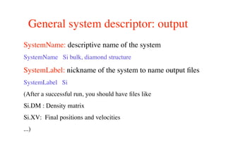
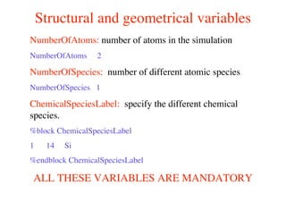
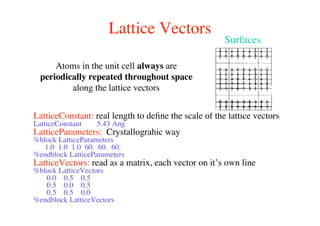
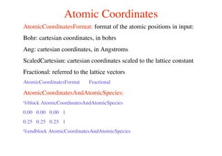
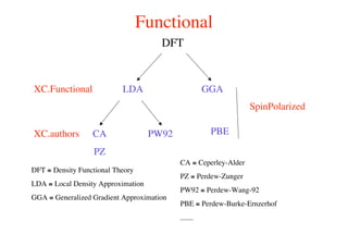
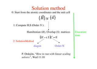
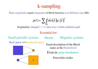
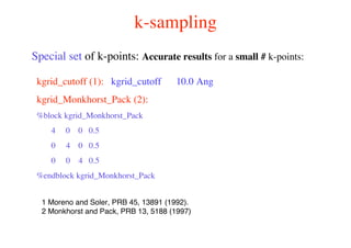
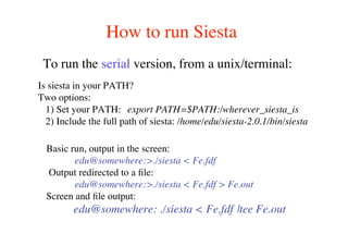
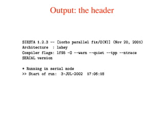
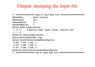
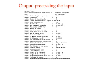
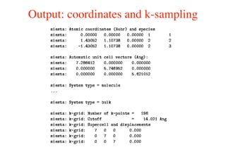
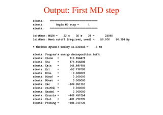
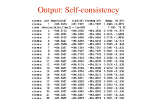
The document provides an introduction to running the Siesta software package for performing density functional theory (DFT) calculations. It describes the basic input variables needed, including system descriptors, structural parameters, functional and basis set specifications. It also outlines how to run Siesta from the command line and analyze outputs such as electronic band structures, densities of states, and charge densities. Post-processing tools are also summarized.

1. Basic introduction to running Siesta
Eduardo Anglada
Siesta foundation-UAM-Nanotec
eduardo.anglada@uam.es
eduardo.anglada@nanotec.es

2. Our method
Linear-scaling DFT based on
NAOs (Numerical Atomic Orbitals)
P. Ordejon, E. Artacho & J. M. Soler , Phys. Rev. B 53, R10441 (1996)
J. M.Soler et al, J. Phys.: Condens. Matter 14, 2745 (2002)
•Born-Oppenheimer (relaxations, mol.dynamics)
•DFT (LDA, GGA)
•Pseudopotentials (norm conserving,factorised)
•Numerical atomic orbitals as basis (finite range)
•Numerical evaluation of matrix elements (3Dgrid)
Implemented in the SIESTA method:
D. Sanchez-Portal, P. Ordejon, E. Artacho & J. M. Soler
Int. J. Quantum Chem. 65, 453 (1997)

3. Siesta resources (I)
•Web page: http://www.uam.es/siesta
•Pseudos and basis database
•Mailing list
•Usage manual
•Soon: http://cygni.fmc.uam.es/mediawiki
•Issue tracker (for bugs, etc)
•Mailing list archives
•Wiki

4. 4
Siesta resources (2)
• Andrei Postnikov Siesta utils page:
http://www.home.uni-
osnabrueck.de/apostnik/download.html
•Lev Kantorovich Siesta utils page:
http://www.cmmp.ucl.ac.uk/~lev/codes/lev00/ind
ex.html

5. Siesta software package:
•Src: Sources of the Siesta code.
•Src/Sys: makefiles for the compilation
•Src/Tests: A collection of tests.
•Docs: Documentation and user conditions:
•User’s Guide (siesta.tex)
•Pseudo: ATOM program to generate and test pseudos.
(A. García; Pseudopotential and basis generation, Tu 11:10)
•Examples: fdf and pseudos input files for simple systems.
•Tutorials: Tutorials for basis and pseudo generation.
•Utils: Programs or scripts to analyze the results.

6. To run Siesta you need:
1.- Access to the executable file: T. White: “And now that
you are back at home ... what?” Friday 13:00.
2.- An input file: written in ascii (plain text) using:
Flexible Data Format (FDF) (A. García and J. M. Soler)
3.- A pseudopotential file for each kind of element in the
input file. Two different formats:
Unformatted binary (.vps)
Formatted ASCII (.psf) (more transportable and easy to look at)

7. Running siesta
Main input file: “name”.fdf
•Contents:
•Physical data of the system
•Variables to control the aproximations
•Format:
•Flexible Data Format (FDF) developed by A. García and J.
M. Soler
Siesta has no windows, it is run from a UNIX terminal or from a
MSDOS console.

8. FDF (I)
•Data can be given in any order
•Data can be omitted in favor of default values
•Syntax: ‘data label’ followed by its value
Character string: SystemLabel h2o
Integer: NumberOfAtoms 3
Real: PAO.SplitNorm 0.15
Logical: SpinPolarized .false.
Physical magnitudes LatticeConstant 5.43 Ang

9. FDF (II)
• Labels are case insensitive and characters -_. are ignored
LatticeConstant is equivalent to lattice_constant
• Text following # are comments
• Logical values: T , .true. , yes, F , .false. , no
By default logicals are true: DM.UseSaveDM
• Character strings, NOT in apostrophes
• Complex data structures: blocks
%block label
…
%endblock label

10. FDF (III)
• Physical magnitudes: followed by its units.
Many physical units are recognized for each magnitude
(Length: m, cm, nm, Ang, bohr)
Automatic conversion to the ones internally required.
• You may ‘include’ other FDF files or redirect the search
to another file, so for example in the main fdf it’s possible:
AtomicCoordinatesFormat < system_xyz.fdf
AtomicCoordinatesAndAtomicSpecies < system_xyz.fdf

11. Basic input variables
1.- General system descriptors
2.- Structural and geometrical variables
3.- Functional and solution mehod (Order-N/diagonalization)
4.- Convergence of the results
5.- Self-consistency
6.- Basis set generation related variables:
“How to test and generate basis sets”, Tu 12:00

12. General system descriptor: output
SystemName: descriptive name of the system
SystemName Si bulk, diamond structure
SystemLabel: nickname of the system to name output files
SystemLabel Si
(After a successful run, you should have files like
Si.DM : Density matrix
Si.XV: Final positions and velocities
...)

13. Structural and geometrical variables
NumberOfAtoms: number of atoms in the simulation
NumberOfAtoms 2
NumberOfSpecies: number of different atomic species
NumberOfSpecies 1
ChemicalSpeciesLabel: specify the different chemical
species.
%block ChemicalSpeciesLabel
1 14 Si
%endblock ChemicalSpeciesLabel
ALL THESE VARIABLES ARE MANDATORY

14. Lattice Vectors
LatticeConstant: real length to define the scale of the lattice vectors
LatticeConstant 5.43 Ang
LatticeParameters: Crystallograhic way
%block LatticeParameters
1.0 1.0 1.0 60. 60. 60.
%endblock LatticeParameters
LatticeVectors: read as a matrix, each vector on it’s own line
%block LatticeVectors
0.0 0.5 0.5
0.5 0.0 0.5
0.5 0.5 0.0
%endblock LatticeVectors
Atoms in the unit cell always are
periodically repeated throughout space
along the lattice vectors
Surfaces

15. Atomic Coordinates
AtomicCoordinatesFormat: format of the atomic positions in input:
Bohr: cartesian coordinates, in bohrs
Ang: cartesian coordinates, in Angstroms
ScaledCartesian: cartesian coordinates scaled to the lattice constant
Fractional: referred to the lattice vectors
AtomicCoordinatesFormat Fractional
AtomicCoordinatesAndAtomicSpecies:
%block AtomicCoordinatesAndAtomicSpecies
0.00 0.00 0.00 1
0.25 0.25 0.25 1
%endblock AtomicCoordinatesAndAtomicSpecies

16. Functional
DFT
XC.Functional LDA GGA
XC.authors PW92CA
PZ
PBE
DFT ≡ Density Functional Theory
LDA ≡ Local Density Approximation
GGA ≡ Generalized Gradient Approximation
CA ≡ Ceperley-Alder
PZ ≡ Perdew-Zunger
PW92 ≡ Perdew-Wang-92
PBE ≡ Perdew-Burke-Ernzerhof
.......
SpinPolarized

17. Solution method
Hamiltonian (H), Overlap (S) matrices
1: Compute H,S (Order N ):
2: SolutionMethod
diagon Order-N
0: Start from the atomic coordinates and the unit cell
P. Ordejón, “How to run with linear-scaling
solvers”, Wed 11:10
Execution
time

18. k-sampling
Many magnitudes require integration of Bloch functions over Brillouin zone (BZ)
!
r
r( ) = d
r
kn
r
k( )
BZ
"i
# $i
r
k( )
2
In practice: integral → sum over a finite uniform grid
Essential for:
Real space ↔Reciprocal space
Small periodic systems Metals Magnetic systems
Good description of the Bloch
states at the Fermi level
Even in same insulators:
Perovskite oxides

19. k-sampling
kgrid_cutoff (1): kgrid_cutoff 10.0 Ang
kgrid_Monkhorst_Pack (2):
%block kgrid_Monkhorst_Pack
4 0 0 0.5
0 4 0 0.5
0 0 4 0.5
%endblock kgrid_Monkhorst_Pack
Special set of k-points: Accurate results for a small # k-points:
1 Moreno and Soler, PRB 45, 13891 (1992).
2 Monkhorst and Pack, PRB 13, 5188 (1997)

20. Selfconsistency (SCF)
Initial guess: !
r
r( )= !atom r
r( )"
!
r
r( ) = !µ,"#µ#"
µ,"
$
Properties: Total energy, Charge density Forces
MaxSCFIterations
Tolerance
Yes
No
?

21. How to run Siesta
To run the serial version, from a unix/terminal:
Basic run, output in the screen:
edu@somewhere:>./siesta < Fe.fdf
Output redirected to a file:
edu@somewhere:>./siesta < Fe.fdf > Fe.out
Screen and file output:
edu@somewhere: ./siesta < Fe.fdf |tee Fe.out
Is siesta in your PATH?
Two options:
1) Set your PATH: export PATH=$PATH:/wherever_siesta_is
2) Include the full path of siesta: /home/edu/siesta-2.0.1/bin/siesta

22. Output: the header

23. Output: dumping the input file

24. Output: processing the input

25. Output: coordinates and k-sampling

26. Output: First MD step

27. Output: Self-consistency

28. Output: Eigenvalues, forces, stress

29. Output: Total energy

30. Output: timer (real and cpu times)

31. Saving and reading information (I)
Some information is stored by Siesta to restart simulations from:
•Density matrix: DM.UseSaveDM
•Localized wave functions (Order-N): ON.UseSaveLWF
•Atomic positions and velocities: MD.UseSaveXV
•Conjugent gradient history (minimizations): MD.UseSaveCG
All of them are logical variables
EXTREMLY USEFUL TO SAVE LOT OF TIME!

32. Saving and reading information (II)
Information needed as input for various post-processing programs, for
example, to visualize:
•Total charge density: SaveRho
•Deformation charge density: SaveDeltaRho
•Electrostatic potential: SaveElectrostaticPotential
•Total potential: SaveTotalPotential
•Local density of states: LocalDensityOfStates
•Charge density contours: WriteDenchar
•Atomic coordinates: WriteCoorXmol and WriteCoorCerius
All of them are logical variables

33. Analyzing the electronic structure (I)
•Band structure along the high symetry lines of the BZ
BandLineScale: scale of the k vectors in BandLines
BandLineScale pi/a
BandLines: lines were band energies are calculated.
%block BandLines
1 1.000 1.000 1.000 L
20 0.000 0.000 0.000 Gamma
25 2.000 0.000 0.000 X
30 2.000 2.000 2.000 Gamma
%endblock BandLines

34. Analyzing the electronic structure (II)
•Density of states: total and projected on the atomic
orbitals
- Compare with experimental spectroscopy
- Bond formation
- Defined as:
ProjectedDensityOfStates:
%block ProjectedDensityOfStates
-20.00 10.00 0.200 500 eV
%endblock ProjectedDensityOfStates

35. Analyzing the electronic structure (III)
•Population analysis: Mulliken prescription
- Amounts of charge on an atom or in an orbital inside
the atom
- Bond formation
- Be careful, very dependent on the basis functions
WriteMullikenPop
WriteMullikenPop 0 = None
1 = Atomic and orbitals charges
2 = 1 + atomic overlap pop.
3 = 2 + orbital overlap pop.

36. Tools (I)
•Various post-processing programs:
-PHONONS:
-Finite differences: VIBRA (P. Ordejón)
-Linear response: LINRES ( J. M. Alons-Pruneda et al.)
-Interphase with Phonon program (Parlinsky)
-Visualize of the CHARGE DENSITY and POTENTIALS
-3D: PLRHO (J. M. Soler)
-2D: CONTOUR (E. Artacho)
-2D: DENCHAR (J. Junquera)
-3D: sies2xsf (Xcrysden) (A. Postnikov: Friday 11:15)
-3D: grid2cube (Gaussian) (P. Ordejón)
-3D: rho2grd (Materials Studio) (O. Paz)

37. Tools (II)
-TRANSPORT PROPERTIES:
-TRANSIESTA (M. Brandbydge et al.)
-PSEUDOPOTENTIAL and BASIS information:
-PyAtom (A. García)
-ATOMIC COORDINATES:
-Sies2arc (J. Gale)
- DOS, PDOS, Bands:
-PlotUtils (O. Paz)