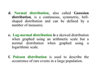
This document provides an overview of biostatistics and descriptive statistics. It defines key biostatistics concepts like data, distributions, and descriptive statistics. It explains how to display data through tables, graphs, and numerical summaries. These include frequency distribution tables, pie charts, bar diagrams, histograms, and more. Descriptive statistics are used to numerically summarize and describe data through measures of central tendency and dispersion.


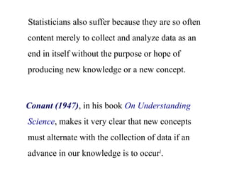
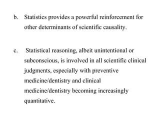
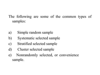
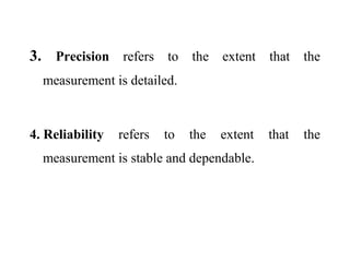

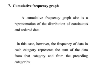
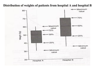
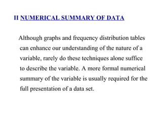
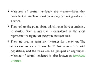
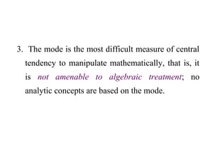
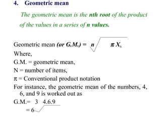
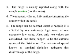
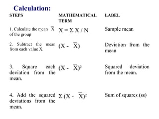
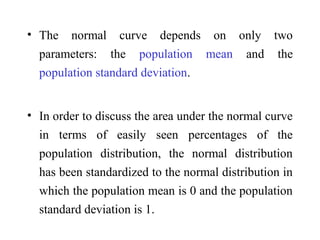
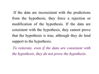
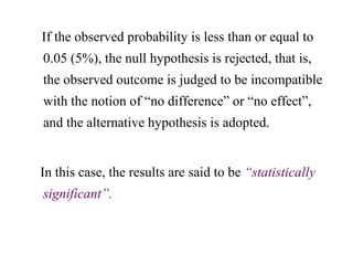
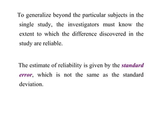
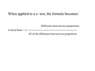
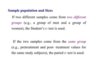
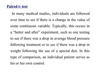
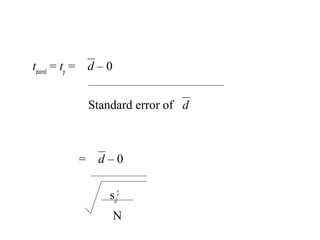
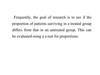
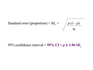
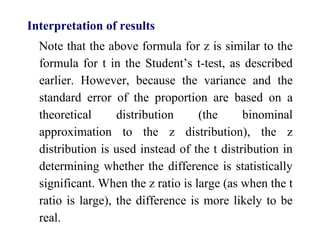
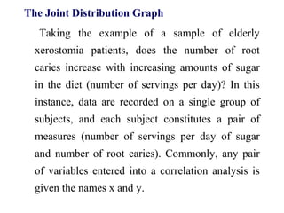
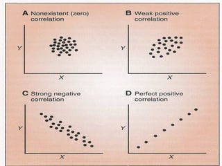
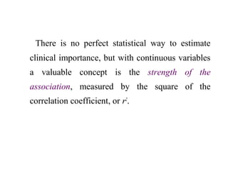
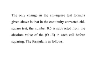
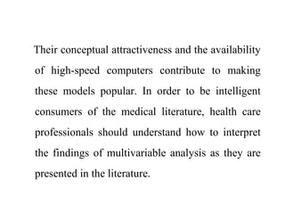
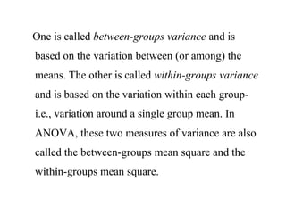
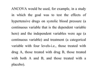
![8. Box plot
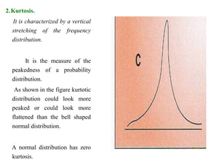
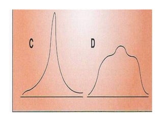
A box plot is a representation of the quartiles
[25%, 50% (median), and 75%] and the range of
a continuous and ordered data set.
The y-axis can be arthimetic or logarithmic.
Box plots can be used to compare the different
distributions of data values.](https://image.slidesharecdn.com/bioppt-160110044607/85/Biostatics-ppt-75-320.jpg)
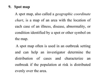
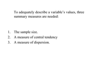

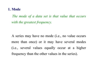
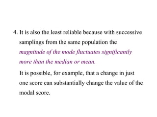
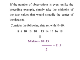

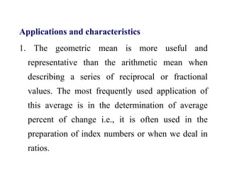
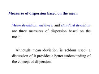
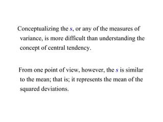
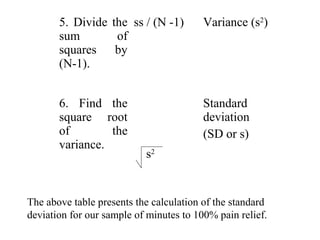
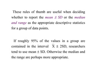
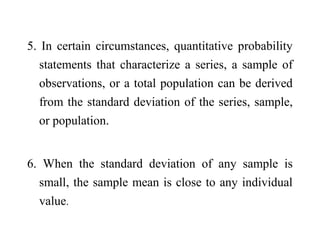

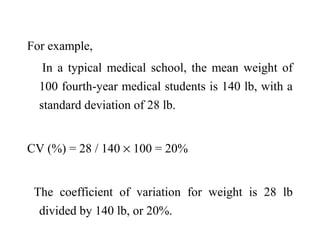
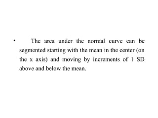
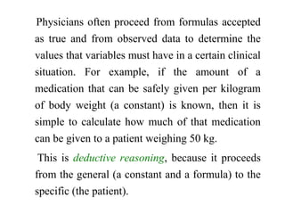
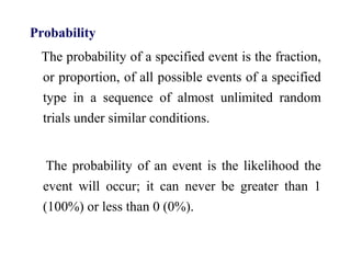
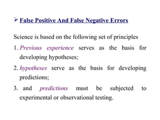
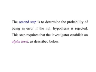
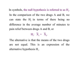

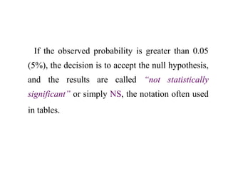
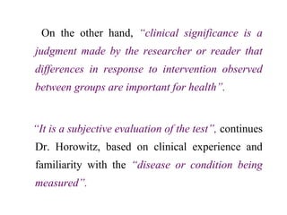
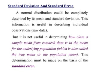
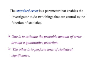
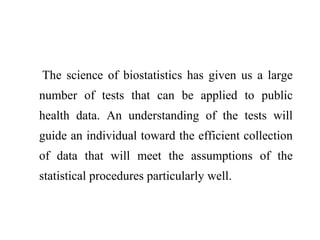
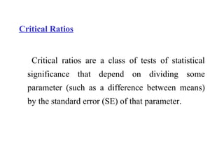
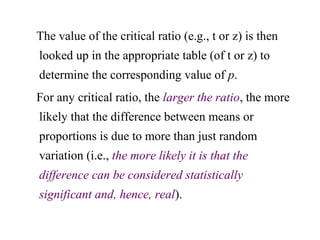
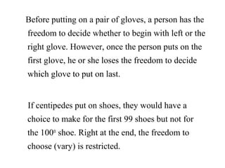
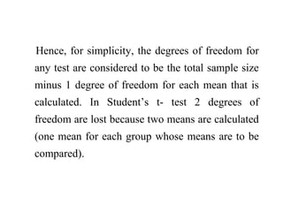
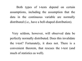
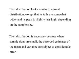
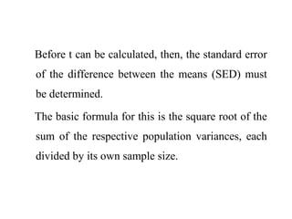
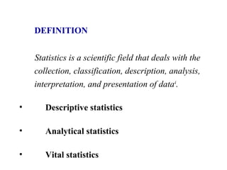
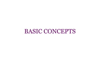
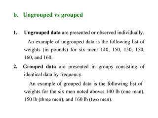
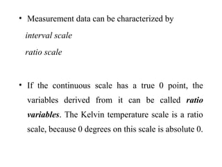
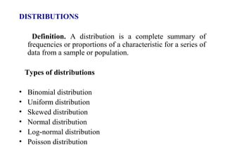
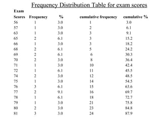
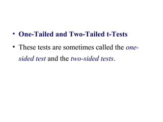
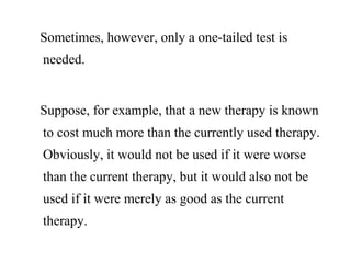
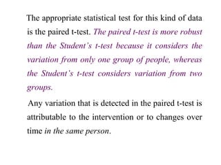
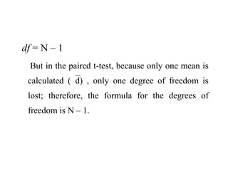
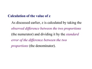
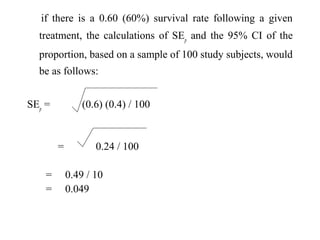
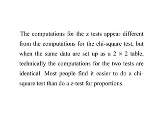
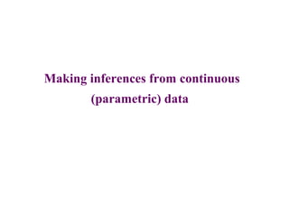
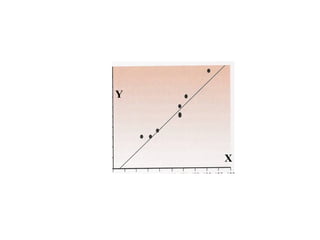
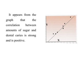
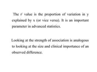
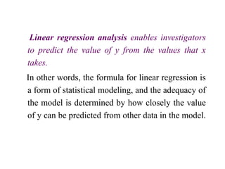
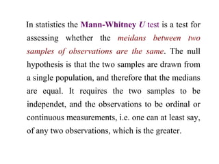
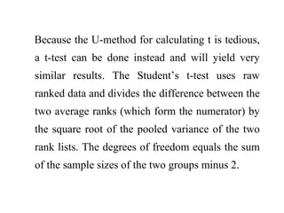
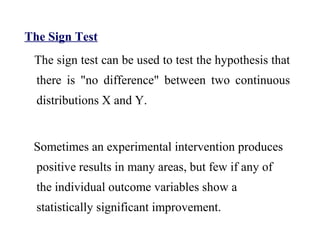
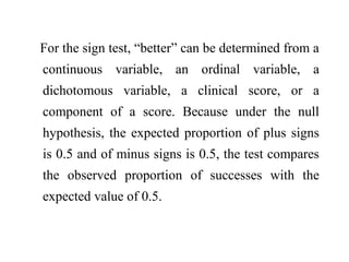
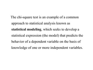
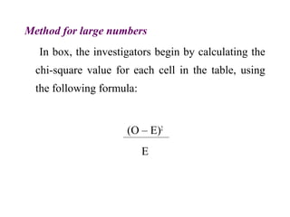
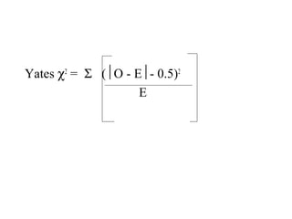
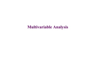
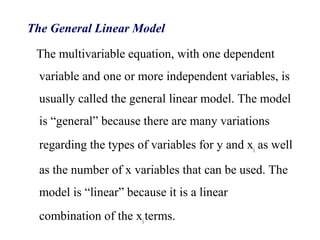
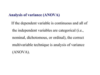
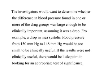
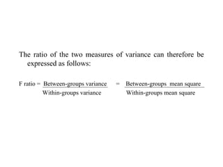
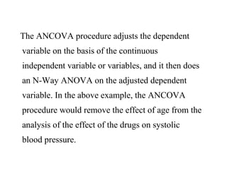
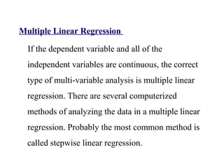
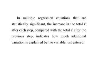
![When the Student’s t-test is used to test the null hypothesis
in research involving an experimrntal group and a control
group, it usually takes the general form of the following
equation:
t = xE
- xC
– 0
s2
p
[(1 / NE
) + (1 / NC
)]
df = NE
+ NC
– 2](https://image.slidesharecdn.com/bioppt-160110044607/85/Biostatics-ppt-286-320.jpg)
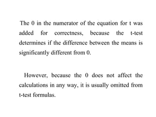
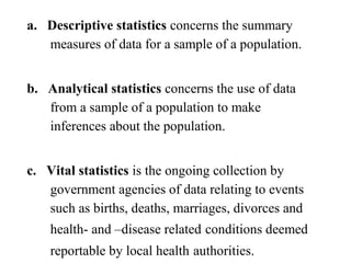
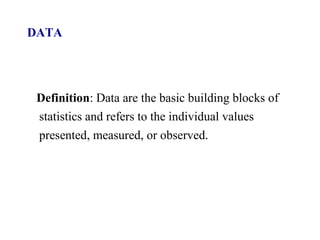
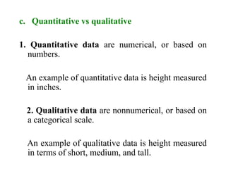
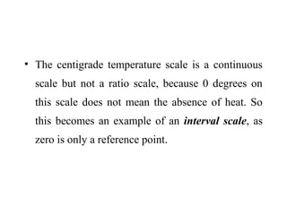
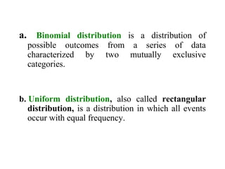
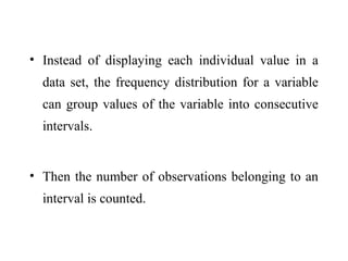
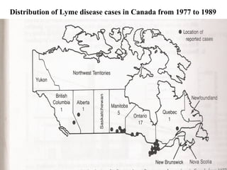
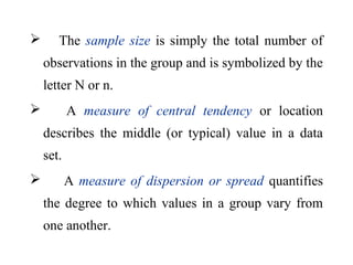
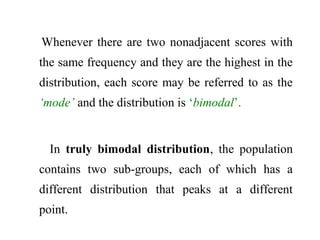
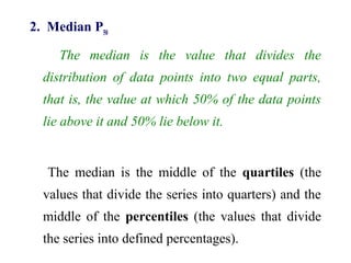
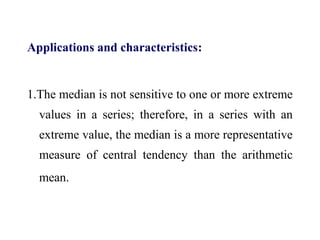
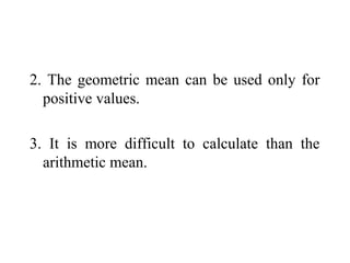
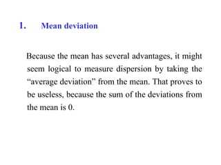
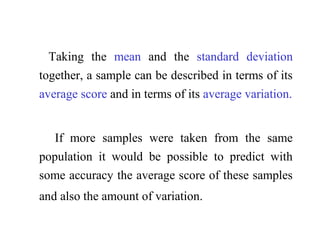
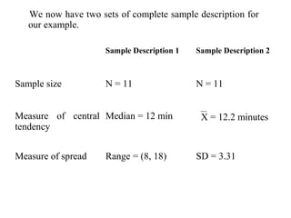
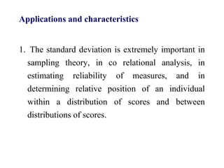
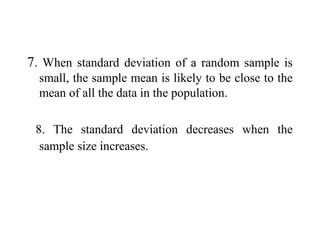
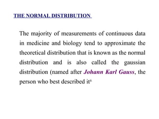
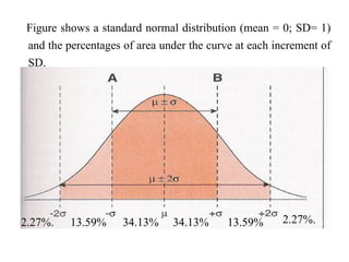
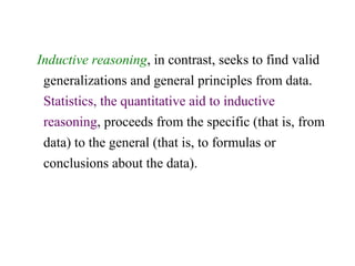
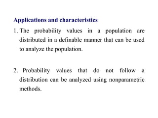
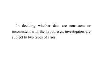
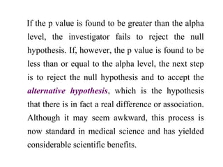
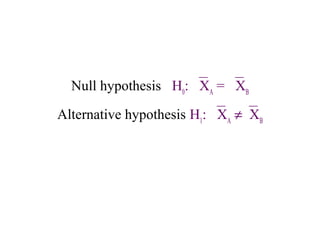
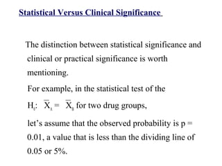
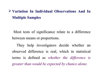
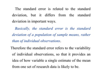
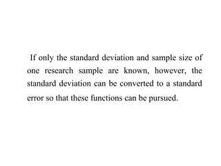
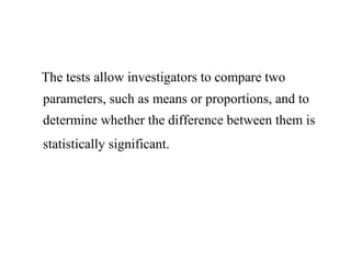
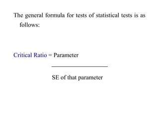
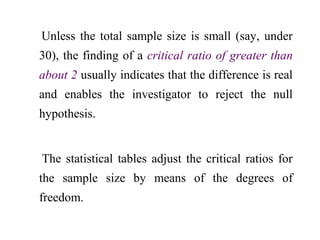
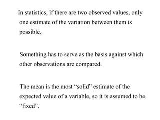
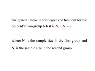
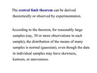
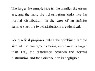
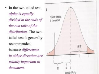
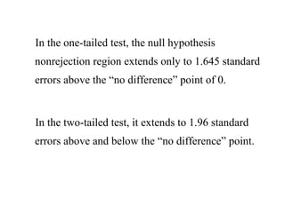
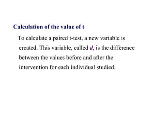
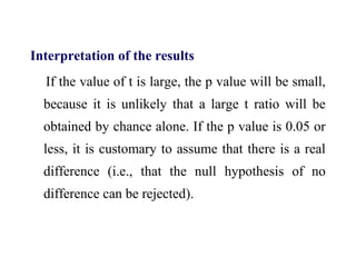
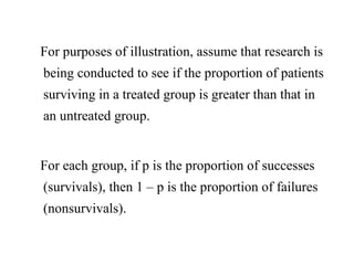
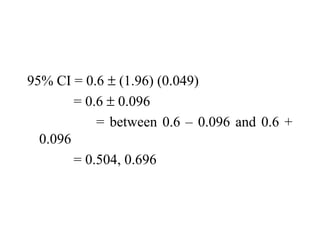
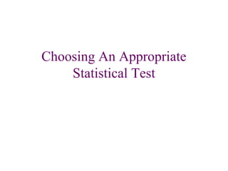
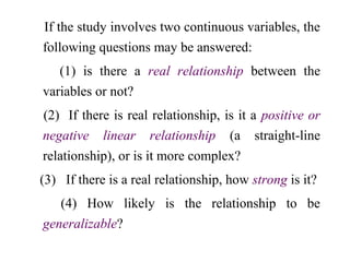
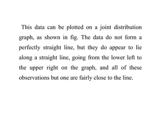
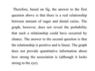
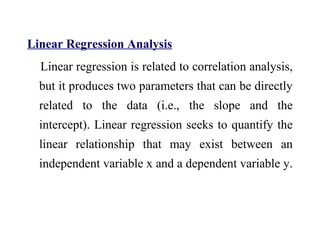
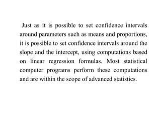
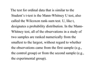
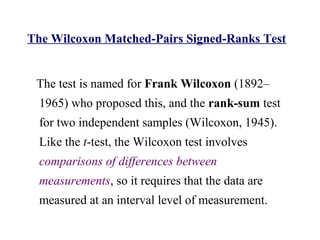
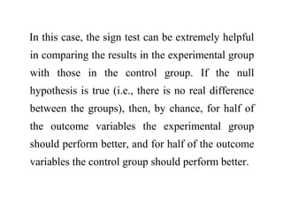
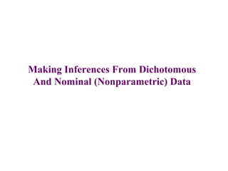
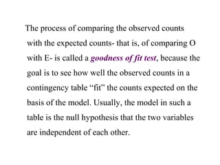
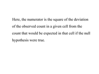
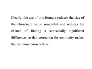
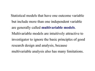
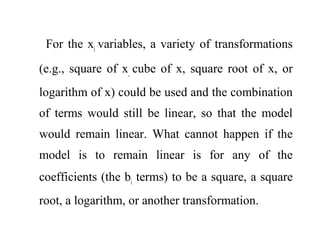
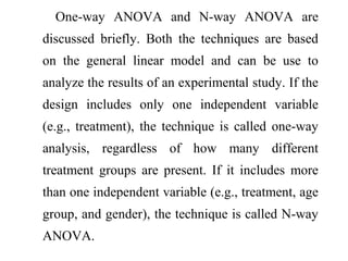
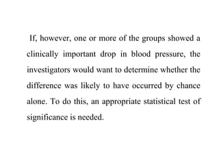
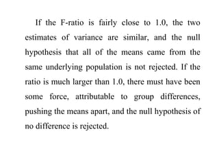
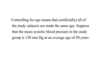
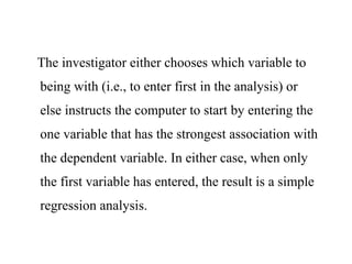
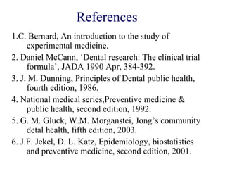
![The same formula, recast in terms to apply to any
two independent samples (e.g., samples of men
and women), is as follows,
t = x1
- x2
- 0
s2
p
[(1 / N1
) + (1 / N2
)]
df = N1
+ N2
– 2](https://image.slidesharecdn.com/bioppt-160110044607/85/Biostatics-ppt-288-320.jpg)
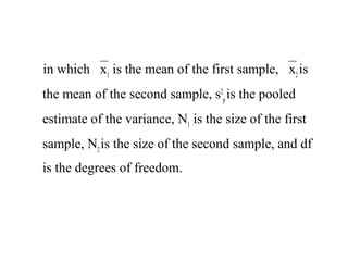
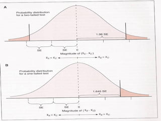

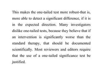
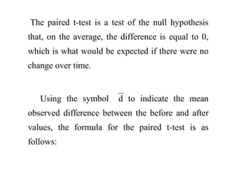
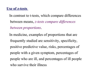
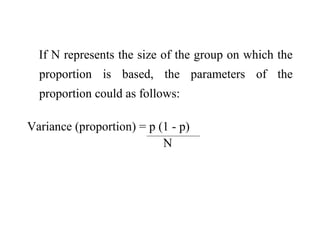
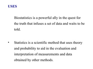
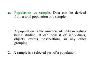
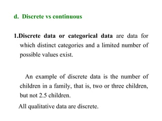
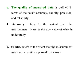
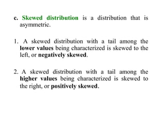
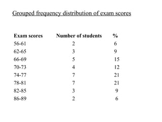
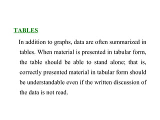
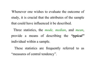
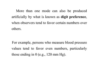
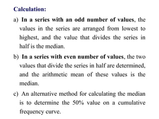
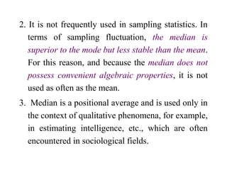
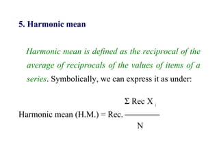
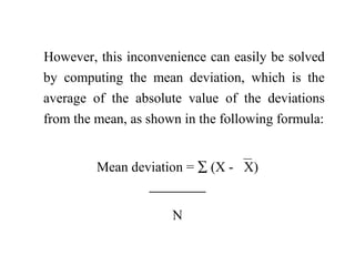
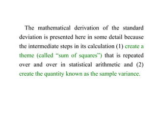
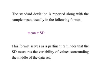
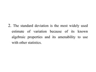
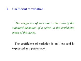
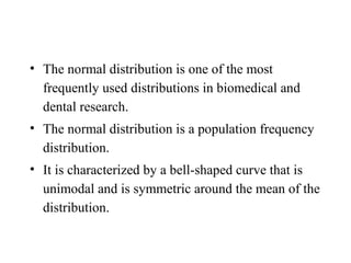
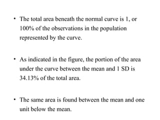
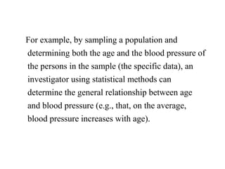
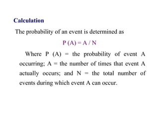
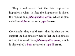
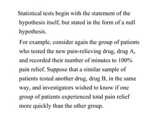
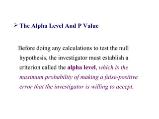
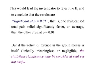
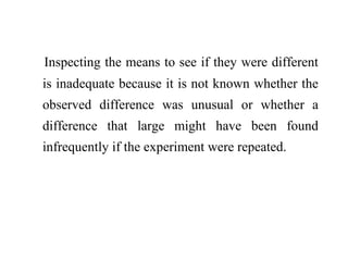
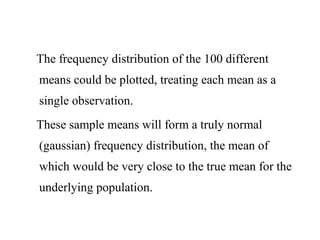
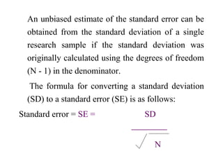
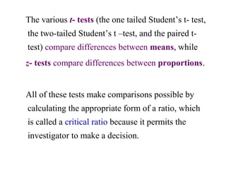
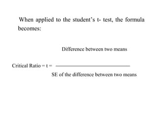
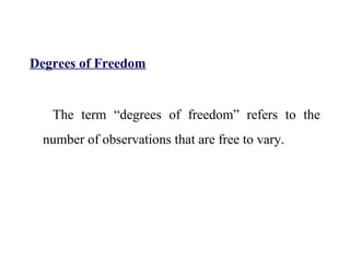
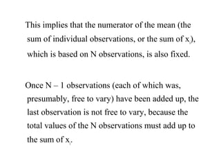
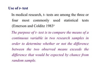
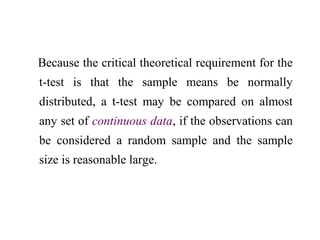
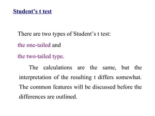
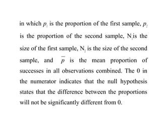
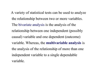
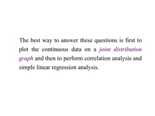
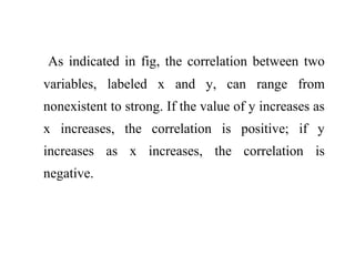
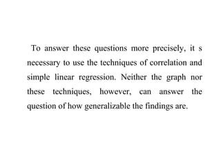
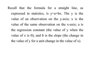
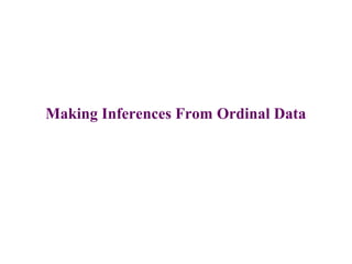
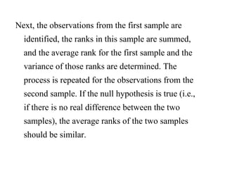
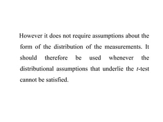
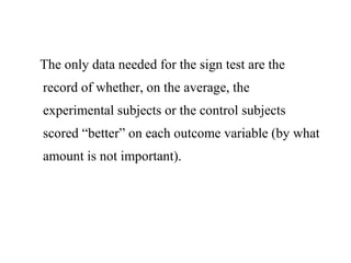
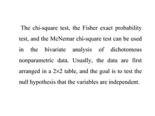
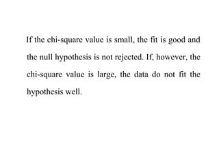
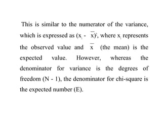
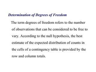
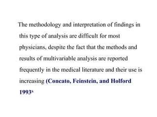
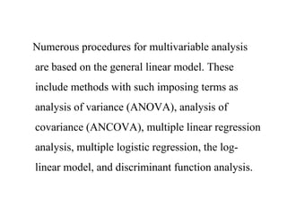
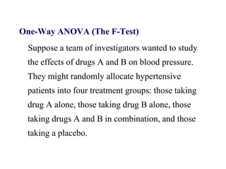
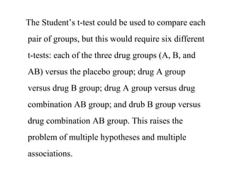
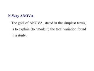
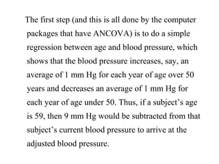
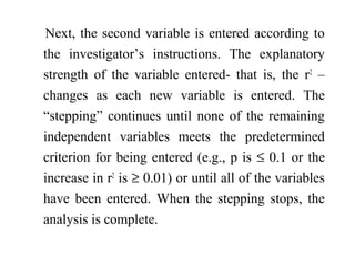
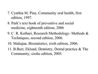
![Now that there is a way to obtain the standard error
of a proportion, the standard error of the
difference between proportions also can be
obtained, and the equation for the z-test can be
expressed as follows:
z = p1
– p2
-0
p (1 - p) [(1/ N1
) + (1/ N2
)]](https://image.slidesharecdn.com/bioppt-160110044607/85/Biostatics-ppt-318-320.jpg)


![7.__Developing_a_Research_Proposal[1].pptx](https://cdn.slidesharecdn.com/ss_thumbnails/7-260131073037-df92dd7d-thumbnail.jpg?width=640&height=640&fit=bounds)


![제 23회 보아즈(BOAZ) 빅데이터 컨퍼런스 - [MBOAX] : ABSA를 활용한 소비자 반응 분석 기반 운영 효율화 대시보드 설계](https://cdn.slidesharecdn.com/ss_thumbnails/3-1boaz23rdconferencemboax-260203102709-9d519923-thumbnail.jpg?width=640&height=640&fit=bounds)