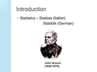
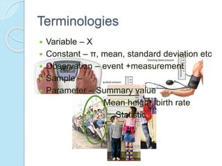
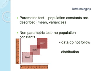
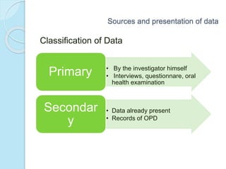
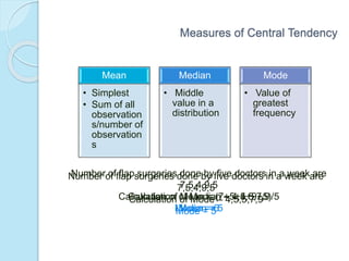
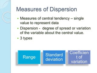
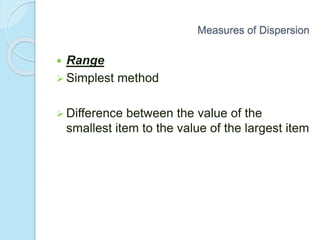
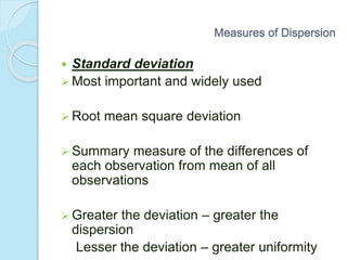
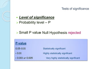
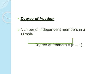
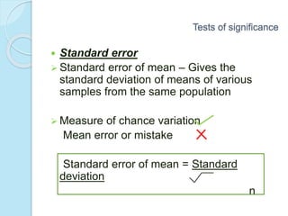
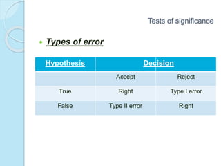
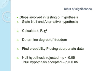
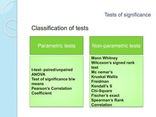
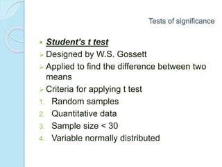
BIOSTATISTICS
Contents
 Introduction
 Terminologies
 Sources & Presentation of Data
 Measures of Central Tendency
 Measures of Dispersion
 Normal curve
 Sampling
 Tests of significance
 Correlation & regression
 Conclusion
Introduction
 Statistics – Statista (Italian)
Statistik (German)
John Graunt
(1620-1674)
Introduction
Why
Statistics?
Epidemiology and Statistics
Introduction
 Variable – X
 Constant – π, mean, standard deviation etc
 Observation – event +measurement
 Sample –
 Parameter – Summary value
Mean height, birth rate
Statistic
Terminologies
Terminologies
 Parametric test – population constants are
described (mean, variances)
 Non parametric test- no population
constants
- data do not follow
specific
distribution
Sources and presentation of data
 Collective recording of observations either
numerical or otherwise.
Sources and presentation of data
• By the investigator himself
• Interviews, questionnare, oral
health examination
Primary
• Data already present
• Records of OPD
Secondar
y
Classification of Data
Sources and presentation of data
 Nominal – Qualitative data
Male / Female
White / Black
Socio- economic status
 Ordinal – Arranged in rank / order
Ramu is taller than Ravi
and Ravi is taller than Ajay
 Interval – Placed in intervals or order
- Uses a scale graded in equal
increments
- Height, weight, blood pressure
 Ratio – Interval scale data is placed with
meaningful ratio
- Biomedically most significant
- Presented in frequency distribution
Qualitative
Quantitative
Sources and presentation of data
Methods of presentation
Tabulation Diagrams
 Tabulation
 Most common way – frequency distribution
table
 Important step in statistical analysis
 Presents a large amount of data – concisely
 Quantitative and qualitative data
Sources and presentation of data
 Diagrams
• Through graphs
• Histogram, frequency polygon,
frequency curve, line graph, scatter or
dot diagram
Quantitative
• Through diagrams
• Bar diagrams, pie diagram, picture
diagram, map diagram
Qualitative
Sources and presentation of data
 Histogram
Teeth
Pocket depth
Pocket depth in five teeth
Sources and presentation of data
2
4
6
 Frequency polygon
0
1
2
3
4
5
6
7
8
1 2 3 4 5 6
Pocket depth
Number of teeth
0
1
2
3
4
5
6
7
8
1 2 3 4 5 6
Sources and presentation of data
0
2000
4000
6000
8000
10000
12000
14000
1999 2003 2007 2011
Numberofpeople
Prevalence of periodontitis in
Belgaum
Sources and presentation of data
Line graph
 Pie Chart
Post graduate students
Orthodontics
Periodontics
Community
dentistry
Prosthodontic
Sources and presentation of data
32% 32 %
23 %13 %
 Bar diagram
Teeth
Pocket depth
Pocket depth in five teeth
Sources and presentation of data
2
4
6
Measures of Central
Tendency
 The single estimate of a series of data that
summarizes the data is known as
parameter.
 Objective : Condense the entire mass of
data
Facilitate comparison
 3 types:
Mean Median Mode
Measures of Central Tendency
Mean
• Simplest
• Sum of all
observation
s/number of
observation
s
Median
• Middle
value in a
distribution
Mode
• Value of
greatest
frequency
Number of flap surgeries done by five doctors in a week are
7,5,4,9,5
Calculation of Mean = (7+5+4+9+5)/5
Mean = 6
Number of flap surgeries done by five doctors in a week are
7,5,4,9,5
Calculation of Median – 4,5,5,7,9
Median = 5
Number of flap surgeries done by five doctors in a week are
7,5,4,9,5
Calculation of Mode – 4,5,5,7,9
Mode = 5
Measures of Dispersion
 Measures of central tendency – single
value to represent data
 Dispersion - degree of spread or variation
of the variable about the central value.
 3 types
Range
Standard
deviation
Coefficien
t of
variation
Measures of Dispersion
 Range
 Simplest method
 Difference between the value of the
smallest item to the value of the largest item
 Standard deviation
 Most important and widely used
 Root mean square deviation
 Summary measure of the differences of
each observation from mean of all
observations
 Greater the deviation – greater the
dispersion
Lesser the deviation – greater uniformity
Measures of Dispersion
 Coefficient of variation
 Standard deviation – deviation within a
series.
 Compare two or more series, with different
units of measurement
Coefficient of variation = Standard deviation
Mean
100
Measures of Dispersion
Normal curve
 Properties
 Bell shaped
 Symmetrical
 Height is maximum
at mean ,
Mean=Median=Mode
 Maximum number of observation at mean
and it decreases on either side
 Relation between mean and standard
deviation
 Forms basis of tests of significance
Normal distribution or Gaussian curve
Sampling
 Need for sampling ??
 Two types of sample selection
Purposive Random
 Sampling techniques
Simple
Random
Systematic
Random
Stratified
Random
Cluster
sampling
Multiphase
sampling
Pathfinder
survey
Sampling
Sampling
1. Simple random sampling
2. Systematic random sampling
 One unit is selected at random and all
other at evenly spaced intervals
 No periodicity of occurrence
Lottery
Table of Random
numbers
3. Stratified Random sampling
 When the population is not homogenous.
 Population is divided in homogenous
groups, followed by simple random
selection
 Merits :
Representative sample from each strata is
secured.
Gives great accuracy
Sampling
 Disadvantage:
Utmost care has to be taken while dividing
the population into strata (regarding
homogeneity of the strata)
Sampling
 Cluster sampling
 Natural clusters – school, village etc.
 From these clusters- the entire population is
surveyed
 Advantages: Simple
Involves less time and cost
 Disadvantage : Higher standard error
Sampling
 Multiphase sampling
 Part of information is collected from whole
sample and a part from sub-sample.
 Advantages : less expensive
less laborious
more purposeful
Sampling
All patients on OPD examined (first phase)
Only those suffering chronic periodontitis
selected (second phase)
Only those within the age group of 35-45
years selected (third phase)
Sample size keeps on becoming smaller
Sampling
 Pathfinder survey
 A specified proportion of the population
 Stratified cluster sampling
 Subjects in specific index age groups are
selected.
 Helps to assess
1. The variations in severity of disease in
different subgroups
2. Picture of age profiles of various oral
diseases.
Sampling
Sample size
 Optimum size of sample based on
following:
1. Approximate idea of estimate of
characteristics- Obtained from previous
studies or pilot studies prior to starting
study.
2. Knowledge about the estimate of
precision – probability level for precision.
Sampling
precision= √n / s (s=SD)
 Sample size
n = Sample size,
p = Approx prevalence rate,
L = Permissible error in p estimation,
Z α = Normal value for probability level.
Sampling
Zα
2 * p * (1-p)
L2
n =
 If p = 10% , investigator allows an error of
prevalence rate of 20%,
n =900
Sampling
4* 0.1*(0.9)
(0.01)2
n =
Tests of significance
 Sampling variability
 Tests of hypothesis
Tests of significance
 Null Hypothesis and Alternative
Hypothesis
Null hypothesis
• No real
difference
• Difference
found -
accidental
Alternative
hypothesis
• Real difference
present
 Level of significance
 Probability level – P
 Small P value
Tests of significance
– Null Hypothesis rejected
P-value
0.05-0.01 Statistically significant
< 0.01 Highly statistically significant
< 0.001 or 0.005 Very highly statistically significant
 Degree of freedom
 Number of independent members in a
sample
Degree of freedom = (n – 1)
Tests of significance
 Standard error
 Standard error of mean – Gives the
standard deviation of means of various
samples from the same population
 Measure of chance variation
Mean error or mistake
Standard error of mean = Standard
deviation
n
 Types of error
Hypothesis
Accept Reject
True Right Type I error
False Type II error Right
Decision
Tests of significance
 Steps involved in testing of hypothesis
1. State Null and Alternative hypothesis
2. Calculate t, F, χ2
3. Determine degree of freedom
4. Find probability P using appropriate data
5. Null hypothesis rejected – p < 0.05
Null hypothesis accepted – p > 0.05
Tests of significance
t-test- paired/unpaired
ANOVA
Test of significance b/w
means
Pearson’s Correlation
Coefficient
Mann Whitney
Wilcoxon’s signed rank
test
Mc nemar’s
Kruskal Wallis
Freidman
Kendall’s S
Chi-Square
Fischer’s exact
Spearman’s Rank
Correlation
Parametric tests Non-parametric tests
Tests of significance
Classification of tests
 These are mathematical tests
 They assess the probability of an observed
difference, occurring by chance
 Most commonly used tests are -
Z test, t test, χ2 test
Tests of significance
 Student’s t test
 Designed by W.S. Gossett
 Applied to find the difference between two
means
 Criteria for applying t test
1. Random samples
2. Quantitative data
3. Sample size < 30
4. Variable normally distributed
Tests of significance
 Unpaired t test
 Data of independent observations made on
individuals of two different groups or
samples
 Checks sampling variability between
experimental and control groups
 e.g. checking sampling variability between
SRP+ subgingival irrigation (experimental
group) and SRP alone (control group)
Tests of significance
 Paired t test
 Paired data of independent observations
from one sample only who gives a pair of
observations.
 E.g. sampling variability in the decrease in
the microbial load before and after
administration of antimicrobial therapy.
Tests of significance
 Wilcoxon’s signed rank test
 Developed by Frank Wilcoxon
 Alternative to the Student’s paired t test
Tests of significance
 Analysis of Variance (ANOVA) test
 Compares more than two samples drawn
from corresponding normal population
 E.g : to check if different agents used for
subgingival irrigation have an effect on the
decrease in microbial load.
Use 3 groups (chlorhexidine , saline,
povidone iodine)
Tests of significance
 If the difference between their means is
significant - different agents used do have
different effect on the decrease in microbial
load.
 To assess this difference in means- ANOVA
test is important
Tests of significance
 Chi – square test
 Developed by Karl Pearson
 Data measured - terms of
attributes/qualities- intended to test if
difference is due to sampling variation
 Involves calculation of a quantity
 3 important applications:
1. Proportion
2. Association
3. Goodness of fit
Tests of significance
 E.g. : Two groups are present
Oral hygiene Oral
hygiene
instructions given instructions
not
given
To assess if there is an association between
gingivitis and oral hygiene instructions.
Tests of significance
Correlation and Regression
 Correlation
 The relationship between two quantitatively
measured variables
 Change in the value of one variable, results
in a change in the other
 Magnitude or degree of relationship
between two variables is called correlation
coefficient (r)
Correlation and Regression
Pearson’s correlation coefficient
Variables are normally distributed
(height and weight)
Variables are not normally distributed
(IQ, income)
 Pearson’s correlation coefficient
Correlation and Regression
 Types of correlation
1. r = +1
2. r = - 1
0 < r < 1
4. -1 < r < 0
5. r = 0
1
65
43
2
 Regression
 Regression coefficient – measure of change
in one character (dependent variable - Y) ,
with one unit change in the independent
character (X)
 Denoted by “b”
 Regression line
Correlation and Regression
 Change of dependent variable in linear way
Y = a+bX
Y = dependent variable
a = Y value
b = regression coefficient
X = independent variable
Correlation and Regression
Conclusion
Clinician Facts
Figures
Statistics
References
 B K Mahajan ; Methods in Biostatistics,
6th edition
 Soben Peter ; Essentials of Preventive and
Community dentistry , 2nd edition
 K. Park ; Parks Textbook of Preventive And
Social medicine , 19th edition
biostatistics

biostatistics

  • 1.
  • 2.
    Contents  Introduction  Terminologies Sources & Presentation of Data  Measures of Central Tendency  Measures of Dispersion  Normal curve  Sampling  Tests of significance  Correlation & regression  Conclusion
  • 3.
    Introduction  Statistics –Statista (Italian) Statistik (German) John Graunt (1620-1674)
  • 4.
  • 5.
  • 6.
     Variable –X  Constant – π, mean, standard deviation etc  Observation – event +measurement  Sample –  Parameter – Summary value Mean height, birth rate Statistic Terminologies
  • 7.
    Terminologies  Parametric test– population constants are described (mean, variances)  Non parametric test- no population constants - data do not follow specific distribution
  • 8.
    Sources and presentationof data  Collective recording of observations either numerical or otherwise.
  • 9.
    Sources and presentationof data • By the investigator himself • Interviews, questionnare, oral health examination Primary • Data already present • Records of OPD Secondar y Classification of Data
  • 10.
    Sources and presentationof data  Nominal – Qualitative data Male / Female White / Black Socio- economic status  Ordinal – Arranged in rank / order Ramu is taller than Ravi and Ravi is taller than Ajay
  • 11.
     Interval –Placed in intervals or order - Uses a scale graded in equal increments - Height, weight, blood pressure  Ratio – Interval scale data is placed with meaningful ratio - Biomedically most significant - Presented in frequency distribution
  • 12.
  • 13.
    Sources and presentationof data Methods of presentation Tabulation Diagrams
  • 14.
     Tabulation  Mostcommon way – frequency distribution table  Important step in statistical analysis  Presents a large amount of data – concisely  Quantitative and qualitative data Sources and presentation of data
  • 15.
     Diagrams • Throughgraphs • Histogram, frequency polygon, frequency curve, line graph, scatter or dot diagram Quantitative • Through diagrams • Bar diagrams, pie diagram, picture diagram, map diagram Qualitative Sources and presentation of data
  • 16.
     Histogram Teeth Pocket depth Pocketdepth in five teeth Sources and presentation of data 2 4 6
  • 17.
     Frequency polygon 0 1 2 3 4 5 6 7 8 12 3 4 5 6 Pocket depth Number of teeth 0 1 2 3 4 5 6 7 8 1 2 3 4 5 6 Sources and presentation of data
  • 18.
    0 2000 4000 6000 8000 10000 12000 14000 1999 2003 20072011 Numberofpeople Prevalence of periodontitis in Belgaum Sources and presentation of data Line graph
  • 19.
     Pie Chart Postgraduate students Orthodontics Periodontics Community dentistry Prosthodontic Sources and presentation of data 32% 32 % 23 %13 %
  • 20.
     Bar diagram Teeth Pocketdepth Pocket depth in five teeth Sources and presentation of data 2 4 6
  • 21.
    Measures of Central Tendency The single estimate of a series of data that summarizes the data is known as parameter.  Objective : Condense the entire mass of data Facilitate comparison  3 types: Mean Median Mode
  • 22.
    Measures of CentralTendency Mean • Simplest • Sum of all observation s/number of observation s Median • Middle value in a distribution Mode • Value of greatest frequency Number of flap surgeries done by five doctors in a week are 7,5,4,9,5 Calculation of Mean = (7+5+4+9+5)/5 Mean = 6 Number of flap surgeries done by five doctors in a week are 7,5,4,9,5 Calculation of Median – 4,5,5,7,9 Median = 5 Number of flap surgeries done by five doctors in a week are 7,5,4,9,5 Calculation of Mode – 4,5,5,7,9 Mode = 5
  • 23.
    Measures of Dispersion Measures of central tendency – single value to represent data  Dispersion - degree of spread or variation of the variable about the central value.  3 types Range Standard deviation Coefficien t of variation
  • 24.
    Measures of Dispersion Range  Simplest method  Difference between the value of the smallest item to the value of the largest item
  • 25.
     Standard deviation Most important and widely used  Root mean square deviation  Summary measure of the differences of each observation from mean of all observations  Greater the deviation – greater the dispersion Lesser the deviation – greater uniformity Measures of Dispersion
  • 26.
     Coefficient ofvariation  Standard deviation – deviation within a series.  Compare two or more series, with different units of measurement Coefficient of variation = Standard deviation Mean 100 Measures of Dispersion
  • 27.
    Normal curve  Properties Bell shaped  Symmetrical  Height is maximum at mean , Mean=Median=Mode  Maximum number of observation at mean and it decreases on either side  Relation between mean and standard deviation  Forms basis of tests of significance Normal distribution or Gaussian curve
  • 28.
    Sampling  Need forsampling ??  Two types of sample selection Purposive Random
  • 29.
  • 30.
    Sampling 1. Simple randomsampling 2. Systematic random sampling  One unit is selected at random and all other at evenly spaced intervals  No periodicity of occurrence Lottery Table of Random numbers
  • 31.
    3. Stratified Randomsampling  When the population is not homogenous.  Population is divided in homogenous groups, followed by simple random selection  Merits : Representative sample from each strata is secured. Gives great accuracy Sampling
  • 32.
     Disadvantage: Utmost carehas to be taken while dividing the population into strata (regarding homogeneity of the strata) Sampling
  • 33.
     Cluster sampling Natural clusters – school, village etc.  From these clusters- the entire population is surveyed  Advantages: Simple Involves less time and cost  Disadvantage : Higher standard error Sampling
  • 34.
     Multiphase sampling Part of information is collected from whole sample and a part from sub-sample.  Advantages : less expensive less laborious more purposeful Sampling
  • 35.
    All patients onOPD examined (first phase) Only those suffering chronic periodontitis selected (second phase) Only those within the age group of 35-45 years selected (third phase) Sample size keeps on becoming smaller Sampling
  • 36.
     Pathfinder survey A specified proportion of the population  Stratified cluster sampling  Subjects in specific index age groups are selected.  Helps to assess 1. The variations in severity of disease in different subgroups 2. Picture of age profiles of various oral diseases. Sampling
  • 37.
    Sample size  Optimumsize of sample based on following: 1. Approximate idea of estimate of characteristics- Obtained from previous studies or pilot studies prior to starting study. 2. Knowledge about the estimate of precision – probability level for precision. Sampling precision= √n / s (s=SD)
  • 38.
     Sample size n= Sample size, p = Approx prevalence rate, L = Permissible error in p estimation, Z α = Normal value for probability level. Sampling Zα 2 * p * (1-p) L2 n =
  • 39.
     If p= 10% , investigator allows an error of prevalence rate of 20%, n =900 Sampling 4* 0.1*(0.9) (0.01)2 n =
  • 40.
    Tests of significance Sampling variability  Tests of hypothesis
  • 41.
    Tests of significance Null Hypothesis and Alternative Hypothesis Null hypothesis • No real difference • Difference found - accidental Alternative hypothesis • Real difference present
  • 42.
     Level ofsignificance  Probability level – P  Small P value Tests of significance – Null Hypothesis rejected P-value 0.05-0.01 Statistically significant < 0.01 Highly statistically significant < 0.001 or 0.005 Very highly statistically significant
  • 43.
     Degree offreedom  Number of independent members in a sample Degree of freedom = (n – 1)
  • 44.
    Tests of significance Standard error  Standard error of mean – Gives the standard deviation of means of various samples from the same population  Measure of chance variation Mean error or mistake Standard error of mean = Standard deviation n
  • 45.
     Types oferror Hypothesis Accept Reject True Right Type I error False Type II error Right Decision Tests of significance
  • 46.
     Steps involvedin testing of hypothesis 1. State Null and Alternative hypothesis 2. Calculate t, F, χ2 3. Determine degree of freedom 4. Find probability P using appropriate data 5. Null hypothesis rejected – p < 0.05 Null hypothesis accepted – p > 0.05 Tests of significance
  • 47.
    t-test- paired/unpaired ANOVA Test ofsignificance b/w means Pearson’s Correlation Coefficient Mann Whitney Wilcoxon’s signed rank test Mc nemar’s Kruskal Wallis Freidman Kendall’s S Chi-Square Fischer’s exact Spearman’s Rank Correlation Parametric tests Non-parametric tests Tests of significance Classification of tests
  • 48.
     These aremathematical tests  They assess the probability of an observed difference, occurring by chance  Most commonly used tests are - Z test, t test, χ2 test Tests of significance
  • 49.
     Student’s ttest  Designed by W.S. Gossett  Applied to find the difference between two means  Criteria for applying t test 1. Random samples 2. Quantitative data 3. Sample size < 30 4. Variable normally distributed Tests of significance
  • 50.
     Unpaired ttest  Data of independent observations made on individuals of two different groups or samples  Checks sampling variability between experimental and control groups  e.g. checking sampling variability between SRP+ subgingival irrigation (experimental group) and SRP alone (control group) Tests of significance
  • 51.
     Paired ttest  Paired data of independent observations from one sample only who gives a pair of observations.  E.g. sampling variability in the decrease in the microbial load before and after administration of antimicrobial therapy. Tests of significance
  • 52.
     Wilcoxon’s signedrank test  Developed by Frank Wilcoxon  Alternative to the Student’s paired t test Tests of significance
  • 53.
     Analysis ofVariance (ANOVA) test  Compares more than two samples drawn from corresponding normal population  E.g : to check if different agents used for subgingival irrigation have an effect on the decrease in microbial load. Use 3 groups (chlorhexidine , saline, povidone iodine) Tests of significance
  • 54.
     If thedifference between their means is significant - different agents used do have different effect on the decrease in microbial load.  To assess this difference in means- ANOVA test is important Tests of significance
  • 55.
     Chi –square test  Developed by Karl Pearson  Data measured - terms of attributes/qualities- intended to test if difference is due to sampling variation  Involves calculation of a quantity  3 important applications: 1. Proportion 2. Association 3. Goodness of fit Tests of significance
  • 56.
     E.g. :Two groups are present Oral hygiene Oral hygiene instructions given instructions not given To assess if there is an association between gingivitis and oral hygiene instructions. Tests of significance
  • 57.
    Correlation and Regression Correlation  The relationship between two quantitatively measured variables  Change in the value of one variable, results in a change in the other  Magnitude or degree of relationship between two variables is called correlation coefficient (r)
  • 58.
    Correlation and Regression Pearson’scorrelation coefficient Pearson’s correlation coefficient Variables are normally distributed (height and weight) Variables are not normally distributed (IQ, income)  Pearson’s correlation coefficient
  • 59.
    Correlation and Regression Types of correlation 1. r = +1 2. r = - 1 0 < r < 1 4. -1 < r < 0 5. r = 0 1 65 43 2
  • 60.
     Regression  Regressioncoefficient – measure of change in one character (dependent variable - Y) , with one unit change in the independent character (X)  Denoted by “b”  Regression line Correlation and Regression
  • 61.
     Change ofdependent variable in linear way Y = a+bX Y = dependent variable a = Y value b = regression coefficient X = independent variable Correlation and Regression
  • 62.
  • 63.
    References  B KMahajan ; Methods in Biostatistics, 6th edition  Soben Peter ; Essentials of Preventive and Community dentistry , 2nd edition  K. Park ; Parks Textbook of Preventive And Social medicine , 19th edition

Editor's Notes

  • #11 O – information gives differences in quality but not in quantity I -
  • #12 also known as numeric scale data
  • #15 Presents a large amount of data – concisely at one glance Add diagram from mahajan
  • #22 , one such parameter is measure of central tendency
  • #24 * Gives the distribution of the data
  • #28 Say the first two paras from soben peter
  • #36 Thereby making it less expensive less labourious more purposeful
  • #42 Alt hypo – in case of rejection of null hypo. Difference in CHX and water for irrgation
  • #44 Eg no of quadrants for sx, df= 3 inspite of 4 quadrants
  • #45 Efficacy of CAF in gain in clinical attachemnt level
  • #60 Read from mahajan
  • #61 When we have understood the correlation b/w 2 variables sometimes it becomes necessary to estimate the value of one character (dependent variable) when the value of the other is known. Eg estimate the weight of a pt based on his height. This is done with regression coefficeint. Reg line is an imaginary line which helps us to understand the diff types of correlation.