Statistics and
Biostatistics
Mrs. Khushbu K. Patel
Assistant professor
Shri Sarvajanik Pharmacy College
What is Statistics?
 Different authors have defined statistics differently. The best definition of statistics is given
by Croxton and Cowden according to whom statistics may be defined as the science, which
deals with collection, presentation, analysis and interpretation of numerical data.
 The science and art of dealing with variation in data through collection, classification, and
analysis in such a way as to obtain reliable results. —(John M. Last, A Dictionary of
Epidemiology )
 Branch of mathematics that deals with the collection, organization, and analysis of numerical
data and with such problems as experiment design and decision making. —(Microsoft
Encarta Premium 2009)
 A branch of mathematic staking and transforming
numbers into useful information for decision makers.
 Methods for processing & analyzing numbers
 Methods for helping reduce the uncertainty inherent
indecision making
What is biostatistics?
 It is the science which deals with development and application of
the most appropriate methods for the:
Collection of data.
Presentation of the collected data.
Analysis and interpretation of the results.
Making decisions on the basis of such analysis
 The methods used in dealing with statistics in the fields of medicine,
biology and public health.
Why study statistics?
 Decision Makers Use Statistics To:
 Present and describe data and information properly
 Draw conclusions about large groups of individuals or information
collected from subsets of the individuals or items.
 Improve processes.
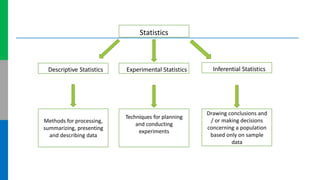
Statistics
Descriptive Statistics Experimental Statistics Inferential Statistics
Methods for processing,
summarizing, presenting
and describing data
Drawing conclusions and
/ or making decisions
concerning a population
based only on sample
data
Techniques for planning
and conducting
experiments
DATA
Definition:-
 A set of values recorded on one or more observational units. Data are
raw materials of statistics.
 Data set : A collection of data is data set
 Data point : A single observation
 Raw data : Information before it arranged and analysed
Sources of data:-
 Experiments
 Surveys
 Records
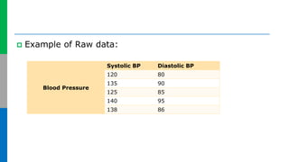
 Example of Raw data:
Blood Pressure
Systolic BP Diastolic BP
120 80
135 90
125 85
140 95
138 86
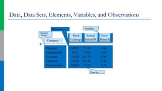
Elements, Variables, and Observations
 The elements are the entities on which data are collected.
 A variable is a characteristic of interest for the elements.
 The set of measurements collected for a particular element is called an
observation.
 The total number of data values in a data set is the number of elements
multiplied by the number of variables.
Data, Data Sets, Elements, Variables, and Observations
Stock
Exchange
Annual
Sales($M)
Earn/
Share($)
Company
V
ariables
Element
Names
Data Set
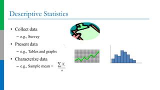
Descriptive statistics
◦ Summarizing and describing the data
◦ Uses numerical and graphical summaries to characterize sample
data
Descriptive Statistics
n
• Collect data
– e.g., Survey
• Present data
– e.g., Tables and graphs
• Characterize data
– e.g., Sample mean =  Xi
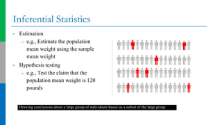
Inferential Statistics
• Estimation
– e.g., Estimate the population
mean weight using the sample
mean weight
• Hypothesis testing
– e.g., Test the claim that the
population mean weight is 120
pounds
Drawing conclusions about a large group of individuals based on a subset of the large group.
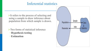
Inferential statistics
It refers to the process of selecting and
using a sample to draw inference about
population from which sample is drawn.
Two forms of statistical inference
◦ Hypothesis testing
◦ Estimation
Basic Vocabulary of Statistics
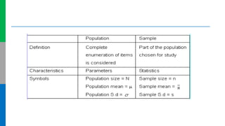
 POPULATION : A population consists of all the items or individuals about which
you want to draw a conclusion. Ex: People who live within 25 kms of radius from
centre of the city.
 SAMPLE : A sample is the portion of a population selected for analysis. It has to be
representative.
 PARAMETER : A parameter is a numerical measure that describes a
characteristic of a population.
 STATISTIC : A statistic is a numerical measure that describes a characteristic of a
sample.
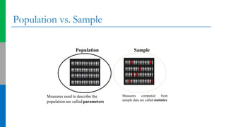
Population vs. Sample
Population Sample
Measures used to describe the
population are called parameters
Measures computed from
sample data are called statistics
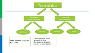
Types of data
Quantitative
data(numerical)
Qualitative
data(categorical)
continuous Discrete Nominal Ordinal
take forever to count
Ex: time
countable in a finite
amount of time
Ex: count change of
money in your pocket
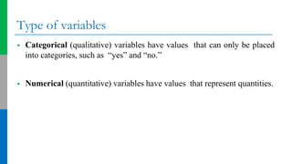
Type of variables
 Categorical (qualitative) variables have values that can only be placed
into categories, such as “yes” and “no.”
 Numerical (quantitative) variables have values that represent quantities.
Qualitative Data
 Non Numerical
 Categorical
 No numbers are use to describe it
 Word, picture, image
 Ex. Do you smoke? Yes No
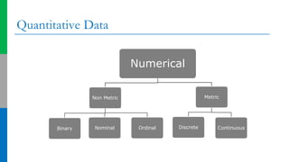
Quantitative Data
Numerical
Non Metric
Binary Nominal Ordinal
Metric
Discrete Continuous
REASONS FOR ASSIGNING NUMBERS
Numbers are usually assigned for two reasons:
 numbers permit statistical analysis of the resulting
data
 numbers facilitate the communication of measurement
rules and results
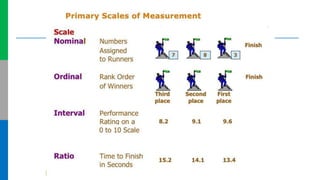
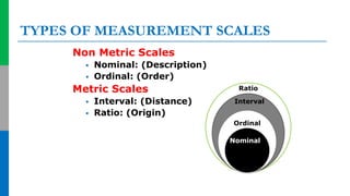
TYPES OF MEASUREMENT SCALES
Non Metric Scales
 Nominal: (Description)
 Ordinal: (Order)
Metric Scales
 Interval: (Distance)
 Ratio: (Origin)
Nominal
Ordinal
Interval
Ratio
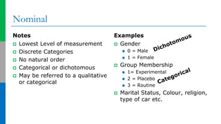
Nominal
Notes
 Lowest Level of measurement
 Discrete Categories
 No natural order
 Categorical or dichotomous
 May be referred to a qualitative
or categorical
Examples
 Gender
 0 = Male
 1 = Female
 Group Membership
 1= Experimental
 2 = Placebo
 3 = Routine
 Marital Status, Colour, religion,
type of car etc.
Nominal
Nominal sounds like name
Notes
 Lowest Level
 Classification of data
 Order is arbitrary
 Gender
 Marital Status
 Religion
 Types of Car Driven
Possible Measures
 Mode
 Model Percentage
 Range
 Frequency Distribution
Ordinal
Notes
 Ordered Categories
 Relative rankings
 Unknown distance between
rankings
 Zero arbitrary
Examples
 Likert Scales
 Socioeconomic status
 Size
 Size, ranking of favorite sports,
class rankings, wellness
rankings
Ordinal
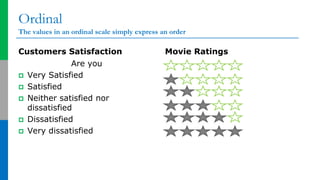
The values in an ordinal scale simply express an order
Customers Satisfaction
Are you
 Very Satisfied
 Satisfied
 Neither satisfied nor
dissatisfied
 Dissatisfied
 Very dissatisfied
Movie Ratings
Ordinal
Notes
 Order matters
 But not the difference between
values
 Unknown distance between
rankings
 Relative rankings
 Likert scales
 Socioeconomic status
 Pain intensity
 Non numeric concepts
Possible Measures
 All Nominal level tests
 Median
 Percentile
 Semi quartile range
 Rank order coefficients of
correlation
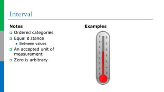
Interval
Notes
 Ordered categories
 Equal distance
 Between values
 An accepted unit of
measurement
 Zero is arbitrary
Examples
Interval
Notes
 Ordered categories
 Equal distance
 Can measure differences
 Zero is arbitrary
 Temperature
 Celsius or Fahrenheit
 Elevation
 Time
Possible Measures
 All Ordinal tests
 Mean
 Standard deviation
 Addition and subtraction
 Can not multiply or divide
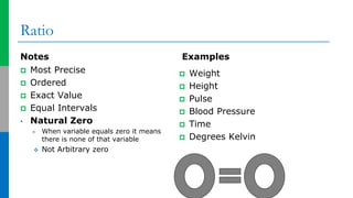
Ratio
Notes
 Most Precise
 Ordered
 Exact Value
 Equal Intervals
• Natural Zero
 When variable equals zero it means
there is none of that variable
 Not Arbitrary zero
Examples
 Weight
 Height
 Pulse
 Blood Pressure
 Time
 Degrees Kelvin
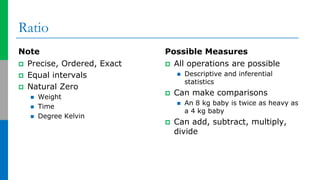
Ratio
Note
 Precise, Ordered, Exact
 Equal intervals
 Natural Zero
 Weight
 Time
 Degree Kelvin
Possible Measures
 All operations are possible
 Descriptive and inferential
statistics
 Can make comparisons
 An 8 kg baby is twice as heavy as
a 4 kg baby
 Can add, subtract, multiply,
divide
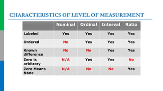
CHARACTERISTICS OF LEVEL OF MEASUREMENT
Nominal Ordinal Interval Ratio
Labeled Yes Yes Yes Yes
Ordered No Yes Yes Yes
Known
difference
No No Yes Yes
Zero is
arbitrary
N/A Yes Yes No
Zero Means
None
N/A No No Yes
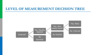
LEVEL OF MEASUREMENT DECISION TREE
Ordered?
Yes, Equally
Spaced
Yes, Zero
means none?
Yes, Ratio
No, Interval
No Ordinal
No
Nominal
Scale
Number
system
Example Permissible
statistics
Nominal
:
Unique definition of
numbers
( 0,1,2,……..9)
Roll number of
students, Numbers
assign to basket ball
players.
Percentages, Mode,
Binomial test, Chi-
Square test
Ordinal:
Order Numbers
(0<1<2……….<9)
Student’s Rank Percentiles, Median,
Rank-order co-
relation, Two-way
ANOVA
Interval
:
Equality of
differences
(2-1 = 7-6)
Temperature Range, Mean,
Standard deviation,
Product Movement
Correlation t- test and
f -test
Ratio:
Equality of Ratio
(5/10 = 3/6)
Weight, height,
distance
Geometric Mean,
Harmonic Mean,
Coefficient of
variation
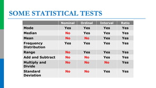
SOME STATISTICAL TESTS
Nominal Ordinal Interval Ratio
Mode Yes Yes Yes Yes
Median No Yes Yes Yes
Mean No No Yes Yes
Frequency
Distribution
Yes Yes Yes Yes
Range No Yes Yes Yes
Add and Subtract No No Yes Yes
Multiply and
Divide
No No No Yes
Standard
Deviation
No No Yes Yes
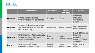
NOIR
Remember Example Central
Tendency
Notes
Nominal
Named classifications;
Mutually exclusive categories
Gender Mode
No order;
Limited in
descriptive
ability
Ordinal
Ordered or Relative rankings;
Numbers are not equidistant;
Zero is arbitrary
Pain scale Mode, median
Not necessarily
equal intervals
Interval
Rank ordering; Approximately
equal intervals; Can have
negative numbers
Exam
marks
Mode,
median, mean
Exact difference
between
numbers is
known; Zero is
arbitrary
Ratio
Rank ordering; Equal
intervals; absolute Zero
Length
Weight
Mode,
Median, Mean
Zero means
none
Methods of presentation of data
1 Tabular presentation
2 Graphical presentation
Purpose: To display data so that they can be readily understood.
Principle: Tables and graphs should contain enough information to be self-
sufficient without reliance on material within the text of the document of which
they are a part.
•Tables and graphs share some common features, but for any specific situation,
one is likely to be more suitable than the other.
Tabular Presentation
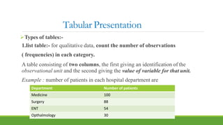
Types of tables:-
1.list table:- for qualitative data, count the number of observations
( frequencies) in each category.
A table consisting of two columns, the first giving an identification of the
observational unit and the second giving the value of variable for that unit.
Example : number of patients in each hospital department are
Department Number of patients
Medicine 100
Surgery 88
ENT 54
Opthalmology 30
Tabular Presentation
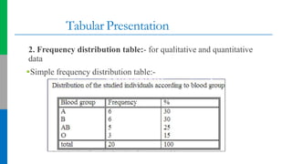
2. Frequency distribution table:- for qualitative and quantitative
data
Simple frequency distribution table:-
Tabular Presentation
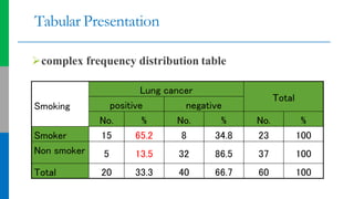
complex frequency distribution table
Smoking
Lung cancer
Total
positive negative
No. % No. % No. %
Smoker 15 65.2 8 34.8 23 100
Non smoker 5 13.5 32 86.5 37 100
Total 20 33.3 40 66.7 60 100
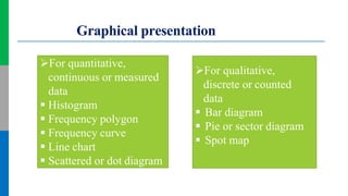
Graphical presentation
For quantitative,
continuous or measured
data
 Histogram
 Frequency polygon
 Frequency curve
 Line chart
 Scattered or dot diagram
For qualitative,
discrete or counted
data
 Bar diagram
 Pie or sector diagram
 Spot map
Bar diagram
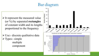
 It represent the measured value
(or %) by separated rectangles
of constant width and its lengths
proportional to the frequency
 Use:- discrete qualitative data
 Types:- simple
multiple
component
Conditions for Which Patients were referred for treatment
0 20 40 80 100 120
B ac k and Neck
A rthritis
A nxiety
Sk in
D igestive
Headache
Gynecologic
Respiratory
Circulatory
General
Blood
Endocrine
Condition
60
N u m b e r of Patients
Bar diagram
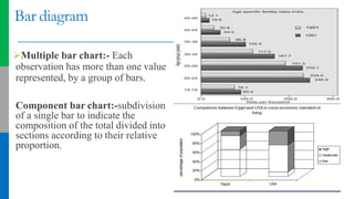
Multiple bar chart:- Each
observation has more than one value
represented, by a group of bars.
Component bar chart:-subdivision
of a single bar to indicate the
composition of the total divided into
sections according to their relative
proportion.
Pie diagram
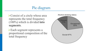
Consist of a circle whose area
represents the total frequency
(100%) which is divided into
segments.
Each segment represents a
proportional composition of the
total frequency
Histogram
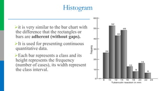
it is very similar to the bar chart with
the difference that the rectangles or
bars are adherent (without gaps).
It is used for presenting continuous
quantitative data.
Each bar represents a class and its
height represents the frequency
(number of cases), its width represent
the class interval.
Frequency polygon
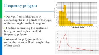
Derived from a histogram by
connecting the mid points of the tops
of the rectangles in the histogram.
The line connecting the centers of
histogram rectangles is called
frequency polygon.
We can draw polygon without
rectangles so we will get simpler form
of line graph
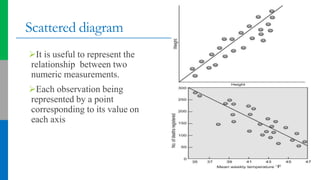
Scattered diagram
It is useful to represent the
relationship between two
numeric measurements.
Each observation being
represented by a point
corresponding to its value on
each axis
Organizing Numerical Data: Frequency
Distribution
 The frequency distribution is a summary table in which the data are
arranged in to numerically ordered classes.
 You must give attention to selecting the appropriate number of class groupings
for the table, determining a suitable width of a class grouping, and establishing
the boundaries of each class grouping to avoid overlapping.
 The number of classes depends on the number of values in the data. With a
larger number of values, typically there are more classes. In general, a
frequency distribution should have at least 5 but no more than 15 classes.
 To determine the width of a class interval, you divide the range (Highest
value–Lowest value) of the data by the number of class groupings desired.
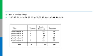
 Example: A manufacturer of insulation randomly selects 20 winter days and records
the daily high temperature
 24, 35, 17, 21, 24, 37, 26, 46, 58, 30, 32, 13, 12, 38, 41, 43, 44, 27, 53, 27
 Sort raw data in ascending order:12, 13, 17, 21, 24, 24, 26, 27, 27, 30, 32,
35, 37, 38, 41, 43, 44, 46, 53, 58
 Find range: 58 -12 = 46
 Select number of classes: 5 (usually between 5 and 15)
 Compute class interval (width): 10 (46/5 then round up)
 Determine class boundaries (limits):
 Class 1: 10 to less than 20
 Class 2: 20 to less than 30
 Class 3: 30 to less than 40
 Class 4: 40 to less than 50
 Class 5: 50 to less than 60
 Compute class midpoints: 15, 25, 35, 45, 55
 Count observations & assign to classes
 Data in ordered array:
 12, 13, 17, 21, 24, 24, 26, 27, 27, 30, 32, 35, 37, 38, 41, 43, 44, 46, 53, 58
1
2
3
4
5
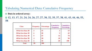
Tabulating Numerical Data: Cumulative Frequency
 Data in ordered array:
 12, 13, 17, 21, 24, 24, 26, 27, 27, 30, 32, 35, 37, 38, 41, 43, 44, 46, 53,
58
Why Use a Frequency Distribution?
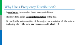
• It condenses the raw data into a more useful form
• It allows for a quick visual interpretation of the data
• It enables the determination of the major characteristics of the data set
including where the data are concentrated / clustered
Frequency Distributions: Some Tips
 Different class boundaries may provide different pictures for
the same data (especially for smaller data sets)
 Shifts in data concentration may show up when different class
boundaries are chosen
 As the size of the data set increases, the impact of alterations
in the selection of class boundaries is greatly reduced
 When comparing two or more groups with different sample
sizes, you must use either a relative frequency or a
percentage distribution
 How to make distribution table ?
https://www.statisticshowto.com/probability-and-
statistics/descriptive-statistics/frequency-distribution-table/
 Online generate frequency distribution
https://www.socscistatistics.com/descriptive/frequencydistribution/de
fault.aspx
 Practice work
https://www.mathsisfun.com/data/frequency-distribution.html
Measures of central tendacy
• The central tendency is the extent to which all the data values group
around a typical or central value.
.
The three most commonly used averages are:
• The arithmetic mean
• The Median
• The Mode
Measures of central tendacy
1. Mean:-
◦ The arithmetic average of the variable x.
◦ It is the preferred measure for interval or ratio variables with relatively
symmetric observations.
◦ It has good sampling stability (e.g., it varies the least from sample to
sample), implying that it is better suited for making inferences about
population parameters.
◦ It is affected by extreme values
Measures of Central Tendency: The Median
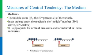
Median:-
The middle value (Q2, the 50th percentile) of thevariable.
In an ordered array, the median is the “middle” number (50%
above, 50% below)
It is appropriate for ordinal measures and for interval or ratio
measures.
• Not affected by extreme values
0 1 2 3 4 5 6 7 8 9 10
Median = 3
0 1 2 3 4 5 6 7 8 9 10
Median = 3
Measures of Central Tendency: The Median
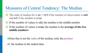
 The rank of median for is (n + 1)/2 if the number of observation is odd
and n/2 if the number is even
 If the number of values is odd, the median is the middle number
 If the number of values is even, the median is the average of the two
middle numbers
Note that is not the value of the median, only the position
of the median in the ranked data.
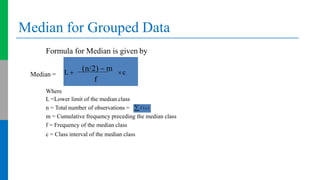
Median for Grouped Data
Formula for Median is given by
Median =
Where
L =Lower limit of the median class
n = Total number of observations =
m = Cumulative frequency preceding the median class
f = Frequency of the median class
c = Class interval of the median class
L 
(n/2)  m c
f
f (x)
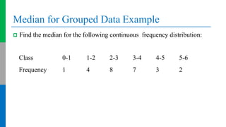
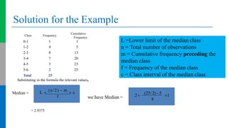
Median for Grouped Data Example
 Find the median for the following continuous frequency distribution:
Class 0-1 1-2 2-3 3-4 4-5 5-6
Frequency 1 4 8 7 3 2
Solution for the Example
Class Frequency
Cumulative
Frequency
0-1 1 1
1-2 4 5
2-3 8 13
3-4 7 20
4-5 3 23
5-6 2 25
Total 25
Substituting in the formula the relevant values,
Median =
= ,
we have Median =
= 2.9375
L 
(n/2)  m
 c
f 2
(25/ 2) 5
1
8
L =Lower limit of the median class
n = Total number of observations
m = Cumulative frequency preceding the
median class
f = Frequency of the median class
c = Class interval of the median class
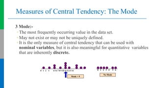
Measures of Central Tendency: The Mode
3 Mode:-
◦ The most frequently occurring value in the data set.
◦ May not exist or may not be uniquely defined.
◦ It is the only measure of central tendency that can be used with
nominal variables, but it is also meaningful for quantitative variables
that are inherently discrete.
0 1 2 3 4 5 6 7 8 9 10 11 12 13 14
Mode = 9
0 1 2 3 4 5 6
No Mode
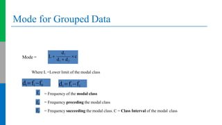
Mode for Grouped Data
Mode =
Where L =Lower limit of the modal class
= Frequency of the modal class
= Frequency preceding the modal class
= Frequency succeeding the modal class. C = Class Interval of the modal class
c
d1
d1  d2
L
d1f1f0 d2 f1f2
f1
f0
f2
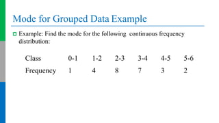
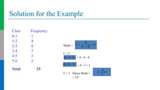
Mode for Grouped Data Example
 Example: Find the mode for the following continuous frequency
distribution:
Class 0-1 1-2 2-3 3-4 4-5 5-6
Frequency 1 4 8 7 3 2
Solution for the Example
Class Frequency
0-1 1
1-2 4
2-3 8
3-4 7
4-5 3
5-6 2
Total 25
Mode =
L = 2
= 8 - 4 = 4
= 8 - 7 = 1
C = 1 Hence Mode =
= 2.8
 c
d1
d1  d2
L 
d1 f1f0
d2 f1 f2
2 
4
1
5
Measure of dispersion
Measures of variability depict how similar observations of a variable tend
to be.
Variability of a nominal or ordinal variable is rarely summarized
numerically.
The measure of dispersion describes the degree of variations or dispersion
of the data around its central values: (dispersion = variation = spread =
scatter).
Range - R
Standard Deviation - SD
Coefficient of Variation -COV
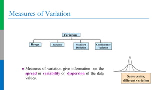
Measures of Variation
Same center,
different variation
 Measures of variation give information on the
spread or variability or dispersion of the data
values.
Variation
Standard
Deviation
Coefficient of
Variation
Range Variance
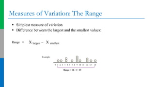
Measures of Variation: The Range
Example:
0 1 2 3 4 5 6 7 8 9 10 11 12 13 14
Range = 14 - 1 = 13
 Simplest measure of variation
 Difference between the largest and the smallest values:
Range = X largest – X smallest
Measure of dispersion
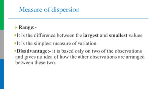
Range:-
It is the difference between the largest and smallest values.
It is the simplest measure of variation.
Disadvantage:- it is based only on two of the observations
and gives no idea of how the other observations are arranged
between these two.
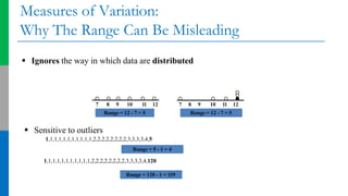
Measures of Variation:
Why The Range Can Be Misleading
 Ignores the way in which data are distributed
7 8 9 10 11 12
Range = 12 - 7 = 5
7 8 9 10 11 12
Range = 12 - 7 = 5
 Sensitive to outliers
1,1,1,1,1,1,1,1,1,1,1,2,2,2,2,2,2,2,2,3,3,3,3,4,5
1,1,1,1,1,1,1,1,1,1,1,2,2,2,2,2,2,2,2,3,3,3,3,4,120
Range = 5 - 1 = 4
Range = 120 - 1 = 119
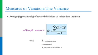
Measures of Variation: The Variance
• Average (approximately) of squared deviations of values from the mean
– Sample variance:
n -1
n
2
 i
(X  X)
S2
 i1
Where X = arithmetic mean
n = sample size
Xi = ith value of the variable X
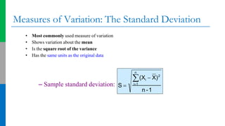
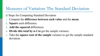
Measures of Variation: The Standard Deviation
• Most commonly used measure of variation
• Shows variation about the mean
• Is the square root of the variance
• Has the same units as the original data
– Sample standard deviation:
n
2
 i
i1
n -1
(X  X)
S 
Measures of Variation: The Standard Deviation
 Steps for Computing Standard Deviation
1. Compute the difference between each value and the mean.
2. Square each difference.
3. Add the squared differences.
4. Divide this total by n-1 to get the sample variance.
5. Take the square root of the sample variance to get the sample standard
deviation.
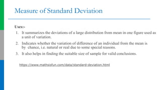
Measure of Standard Deviation
Uses:-
1. It summarizes the deviations of a large distribution from mean in one figure used as
a unit of variation.
2. Indicates whether the variation of difference of an individual from the mean is
by chance, i.e. natural or real due to some special reasons.
3. It also helps in finding the suitable size of sample for valid conclusions.
https://www.mathsisfun.com/data/standard-deviation.html
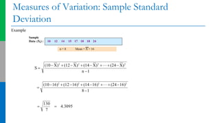
Measures of Variation: Sample Standard
Deviation
Sample
Data (Xi) : 10 12 14 15 17 18 18 24
n = 8 Mean = X = 16
Example
7
130
 4.3095

81

n 1
S 
(1016)2
 (1216)2
 (1416)2
 (2416)2
(10 X)2
 (12 X)2
 (14 X)2
 (24 X)2
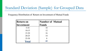
Standard Deviation (Sample) for Grouped Data
Frequency Distribution of Return on Investment of Mutual Funds
Return on
Investment
Number of Mutual
Funds
5-10
10-15
15-20
20-25
25-30
Total
10
12
16
14
8
60
Solution for the Example
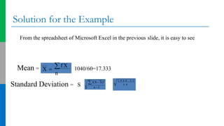
From the spreadsheet of Microsoft Excel in the previous slide, it is easy to see
Mean = = 1040/60=17.333
= = 6.44
Standard Deviation = S
X  f X
n
f(X X)2
n 1
2 4 4 8 . 3 3
5 9
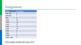
Assignment
Class Frequency
700-799 4
800-899 7
900 8
1000 10
1100 12
1200 17
1300 13
1400 10
1500 9
1600 7
1700 2
1800-1899 1
Find sample standard deviation S.D.
Measures of Variation: Comparing Standard
Deviations
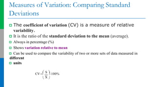
 The coefficient of variation (CV) is a measure of relative
variability.
 It is the ratio of the standard deviation to the mean (average).
 Always in percentage (%)
 Shows variation relative to mean
 Can be used to compare the variability of two or more sets of data measured in
different
 units
 
 S 
CV  100%
X
Measure of dispersion
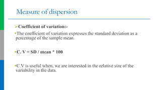
Coefficient of variation:-
The coefficient of variation expresses the standard deviation as a
percentage of the sample mean.
C. V = SD / mean * 100
C.V is useful when, we are interested in the relative size of the
variability in the data.
Measures of Variation: Comparing Standard
Deviations
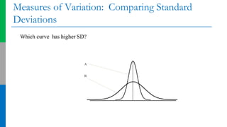
A
B
Which curve has higher SD?
Measures of Variation: Comparing Standard
Deviations
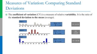
 The coefficient of variation (CV) is a measure of relative variability. It is the ratio of
the standard deviation to the mean (average).
Mean = 15.5
S = 3.338
11 12 13 14 15 16 17 18 19 20 21
11 12 13 14 15 16 17 18 19 20 21
Data B
DataA
Mean = 15.5
S = 0.926
11 12 13 14 15 16 17 18 19 20 21
Mean = 15.5
S = 4.570
Data C
CV =21.53
CV
=5.97
CV =29.48
Measures of Variation: Comparing Coefficients
of Variation
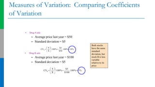
• Drug A sale
– Average price last year = $50
– Standard deviation = $5
• Drug B sale:
– Average price last year = $100
– Standard deviation = $5
$5
X $50
A 100% 10%
100% 
 
 
 S 
CV 
$100
$5
X
B 100% 5%
100%
 
 
 S 
CV 
Both stocks
have the same
standard
deviation, but
stock B is less
variable
relative to its
price
Introduction of biostatistics