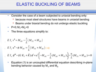
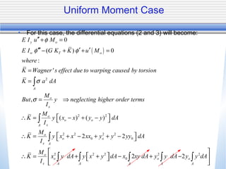
(1) The elastic buckling behavior of beams can be described by three second-order differential equations relating the bending moments and shear and torsional forces. (2) For a beam under uniaxial bending only, the equations simplify to one governing in-plane bending and two coupled equations describing lateral-torsional buckling. (3) For a beam under a uniform moment, the differential equations can be solved analytically, with the critical buckling moment determined by beam properties and dimensions. Numerical methods like the finite difference method are needed to solve for non-uniform moments.

1. Elastic Buckling Behavior of Beams
CE579 - Structural Stability and Design

2. ELASTIC BUCKLING OF BEAMS
• Going back to the original three second-order differential
equations:
( ) ( )
( ) ( )
0
0
0
0
,
( ) ( ( ) )
( ( ) ) ( ) ( ) 0
x BY TY BY BX TX BX
y BX TY BY BY TX BX
w T BX BX TX
BY BY TY TY BY TX BX
Therefore
z z
E I v P v P x M M M M M M
L L
z z
E I u P u P y M M M M M M
L L
z
E I G K K u M M M P y
L
z v u
v M M M P x M M M M
L L L
φ
φ
φ φ
 
′′+ − + − + = − + ÷
 
 ′′+ − − + − + = − + + ÷
 
′′′ ′ ′− + + − − + +
′− + + + − + − + =
1
2
3
(MTX+MBX) (MTY+MBY)

3. ELASTIC BUCKLING OF BEAMS
• Consider the case of a beam subjected to uniaxial bending only:
 because most steel structures have beams in uniaxial bending
 Beams under biaxial bending do not undergo elastic buckling
• P=0; MTY=MBY=0
• The three equations simplify to:
• Equation (1) is an uncoupled differential equation describing in-plane
bending behavior caused by MTX and MBX
( )
( )
( ) ( ) ( ) 0
x BX TX BX
y BX TX BX
w T BX BX TX TX BX
z
E I v M M M
L
z
E I u M M M
L
z u
E I G K K u M M M M M
L L
φ
φ φ
′′ = − +
′′− = +
 
′′′ ′ ′− + + − − + − + = ÷
 
1
2
3
(−φ)

4. ELASTIC BUCKLING OF BEAMS
• Equations (2) and (3) are coupled equations in u and φ – that
describe the lateral bending and torsional behavior of the beam. In
fact they define the lateral torsional buckling of the beam.
• The beam must satisfy all three equations (1, 2, and 3). Hence,
beam in-plane bending will occur UNTIL the lateral torsional
buckling moment is reached, when it will take over.
• Consider the case of uniform moment (Mo) causing compression in
the top flange. This will mean that
 -MBX = MTX = Mo

5. Uniform Moment Case
• For this case, the differential equations (2 and 3) will become:
( )
2
2 2
2 2 2 2
0 0
0
( ) 0
:
'
,
( ) ( )
2 2
y o
w T o
A
o
x
o
o o
xA
o
o o
x
E I u M
E I G K K u M
where
K Wagner s effect due to warping caused by torsion
K a dA
M
But y neglecting higher order terms
I
M
K y x x y y dA
I
M
K y x x xx y y yy dA
I
φ
φ φ
σ
σ
′′+ =
′′′ ′ ′− + + =
=
=
= ⇒
 ∴ = − + − 
 ∴ = + − + + − 
∫
∫
2 2 2 2 2
0 2 2
A
o
o o o
x A A A A A
M
K x y dA y x y dA x xy dA y y dA y y dA
I
 
 ∴ = + + − + −  
 
∫
∫ ∫ ∫ ∫ ∫

6. ELASTIC BUCKLING OF BEAMS
2 2
2 2
2 2
2
2
, 2
sec
o
o x
x A
A
o o
x
A
o x x o
x
x
M
K y x y dA y I
I
y x y dA
K M y
I
y x y dA
K M where y
I
is a new tional property
β β
β
 
 ∴ = + −  
 
  +  
∴ = − 
 
 
 + 
∴ = ⇒ = −
∫
∫
∫
( )
:
(2) 0
(3) ( ) 0
y o
w T o x o
The beam buckling differential equations become
E I u M
E I G K M u M
φ
φ β φ
′′+ =
′′′ ′ ′− + + =

7. ELASTIC BUCKLING OF BEAMS
2
2
2
2
1 2 2
1 2
(2)
(2) (3) :
( ) 0
sec : 0
0
,
0
o
y
iv o
w T o x
y
x
iv oT
w y w
oT
w y w
iv
M
Equation gives u
E I
Substituting u from Equation in gives
M
E I G K M
E I
For doubly symmetric tion
MG K
E I E I I
MG K
Let and
E I E I I
φ
φ β φ φ
β
φ φ φ
λ λ
φ λ φ λ φ
′′ = −
′′
′′− + − =
=
′′∴ − − =
= =
′′∴ − − = ⇒ . .becomes the combined d e of LTB

8. ELASTIC BUCKLING OF BEAMS
( )
1 1 2 2
4 2
1 2
4 2
1 2
2 2
1 1 2 1 2 12
2 2
1 1 2 1 1 2
1 2
1 2 3 4
0
0
4 4
,
2 2
4 4
,
2 2
, ,
z
z
z z i z i z
Assume solution is of the form e
e
i
Let and i
Above are the four roots for
C e C e C e C e
collect
λ
λ
α α α α
φ
λ λ λ λ
λ λ λ λ
λ λ λ λ λ λ
λ
λ λ λ λ λ λ
λ
λ α α
λ
φ − −
=
∴ − − =
∴ − − =
+ + + −
∴ = −
+ + + +
∴ = ± ±
∴ = ± ±
∴ = + + +
∴
1 1 2 1 3 2 4 2cosh( ) sinh( ) sin( ) cos( )
ing real and imaginary terms
G z G z G z G zφ α α α α∴ = + + +

9. ELASTIC BUCKLING OF BEAMS
• Assume simply supported boundary conditions for the beam:
1
2 2
1 2 2
1 1 2 2 3
2 2 2 2
41 1 1 1 2 2 2 2
(0) (0) ( ) ( ) 0
. .
1 0 0 1
0 0
0
cosh( ) sinh( ) sin( ) cos( )
cosh( ) sinh( ) sin( ) cos( )
L L
Solution for must satisfy all four b c
G
G
L L L L G
GL L L L
For buckl
φ φ φ φ
φ
α α
α α α α
α α α α α α α α
′′ ′′∴ = = = =
   
   −  
 × = 
   
   − −   
( )2 2
1 2 1 2
2
2
sin :
det min 0
sinh( ) sinh( ) 0
:
sinh( ) 0
ing coefficient matrix must be gular
er ant of matrix
L L
Of these
only L
L n
α α α α
α
α π
∴ =
∴ + × × =
=
∴ =

10. ELASTIC BUCKLING OF BEAMS
( )
2
2
1 2 1
2
2
1 2 1 2
22 2 2
2
1 1 12 2 2
2
2 2
2 12 2
2 2 2
2 2 2 2
2 2
2
2 2
4
2
2
4
2 2 2
2
4 4
o T
y w w
T
o y w
w
n
L
L
L
L L L
L L
M G K
E I I L E I L
G K
M E I I
L E I L
π
α
λ λ λ π
π
λ λ λ
π π π
λ λ λ
λ
π π
λ λ
π π
λ
π π
∴ =
+ −
∴ =
∴ + − =
    
+ − + ÷  ÷ ÷
    ∴ = =
  
∴ = + ÷ ÷
  
  
∴ = = + ÷ ÷
  
  
∴ = + ÷ ÷
  
2 2
2 2
y w
o T
E I E I
M G K
L L
π π 
∴ = + ÷
 

11. Uniform Moment Case
• The critical moment for the uniform moment case is given by
the simple equations shown below.
• The AISC code massages these equations into different
forms, which just look different. Fundamentally the equations
are the same.
 The critical moment for a span with distance Lb between lateral -
torsional braces.
 Py is the column buckling load about the minor axis.
 Pφ is the column buckling load about the torsional z- axis.
Mcr
o
=
π2
EIy
L2
×
π2
EIw
L2
+GKT






Mcr
o
= Py ×Pφ ×ro
2

12. Non-uniform moment
• The only case for which the differential equations can be
solved analytically is the uniform moment.
• For almost all other cases, we will have to resort to numerical
methods to solve the differential equations.
• Of course, you can also solve the uniform moment case
using numerical methods
( )
( )
( ) ( ) ( ) 0
x BX TX BX
y BX TX BX
w T BX BX TX TX BX
z
E I v M M M
L
z
E I u M M M
L
z u
E I G K K u M M M M M
L L
φ
φ φ
′′ = − +
′′− = +
 
′′′ ′ ′− + + − − + − + = ÷
 
φ

13. What numerical method to use
• What we have is a problem where the governing differential equations are
known.
 The solution and some of its derivatives are known at the boundary.
 This is an ordinary differential equation and a boundary value
problem.
• We will solve it using the finite difference method.
 The FDM converts the differential equation into algebraic equations.
 Develop an FDM mesh or grid (as it is more correctly called) in the
structure.
 Write the algebraic form of the d.e. at each point within the grid.
 Write the algebraic form of the boundary conditions.
 Solve all the algebraic equations simultaneously.

14. Finite Difference Method
f(x+h)= f(x)+h ′f (x)+
h2
2!
′′f (x)+
h3
3!
′′′f (x)+
h4
4!
f iv
(x)+K
∴ ′f (x)=
f(x+h)− f(x)
h
+
h
2!
′′f (x)+
h2
3!
′′′f (x)+
h3
4!
f iv
(x)+K
∴ ′f (x)=
f(x+h)− f(x)
h
+O(h) ⇒Forwarddifferenceequation
h h
f(x)f(x-h)
f
x
f’(x)
Forward difference
Backward difference
Central difference
f(x+h)

15. Finite Difference Method
f (x+h) = f (x)+h ′f (x)+
h2
2!
′′f (x)+
h3
3!
′′′f (x)+
h4
4!
f iv
(x)+K
f (x−h) = f (x)−h ′f (x)+
h2
2!
′′f (x)−
h3
3!
′′′f (x)+
h4
4!
f iv
(x)+K
∴ ′f (x) =
f (x+h)− f (x−h)
2h
+
2h2
3!
′′′f (x)+K
∴ ′f (x) =
f (x+h)− f (x−h)
2h
+O(h2
) ⇒Central differenceequation
f(x−h)= f(x)−h ′f (x)+
h2
2!
′′f (x)−
h3
3!
′′′f (x)+
h4
4!
f iv
(x)+K
∴ ′f (x)=
f(x)− f(x−h)
h
+
h
2!
′′f (x)−
h2
3!
′′′f (x)+
h3
4!
f iv
(x)+K
∴ ′f (x)=
f(x)− f(x−h)
h
+O(h) ⇒Backwarddifferenceequation

16. Finite Difference Method
• The central difference equations are better than the forward
or backward difference because the error will be of the order
of h-square rather than h.
• Similar equations can be derived for higher order derivatives
of the function f(x).
• If the domain x is divided into several equal parts, each of
length h.
• At each of the ‘nodes’ or ‘section points’ or ‘domain points’
the differential equations are still valid.
1 2 3 i-2 i-1 i i+1 i+2 n
h

17. Finite Difference Method
• Central difference approximations for higher order
derivatives: Notation
y = f (x)
yi = f (x =i)
yi
′ = ′f (x =i)
yi
′′ = ′′f (x =i) and soonL
yi
′ =
1
2h
yi+1 − yi−1( )
yi
′′ =
1
h2
yi+1 −2yi + yi−1( )
yi
′′′ =
1
2h3
yi+2 −2yi+1 +2yi−1 − yi−2( )
yi
iv
=
1
h4
yi+2 −4yi+1 +6yi −4yi−1 + yi−2( )

18. FDM - Beam on Elastic Foundation
• Consider an interesting problemn --> beam on elastic
foundation
• Convert the problem into a finite difference problem.
Fixed end Pin support
x L
w(x)=w
K=elastic fdn.
EIyiv
+ky(x)=w(x)
1 2 3 4 5 6
h =0.2 l
EIyi
iv
+kyi=w
Discrete form of differential equation

19. FDM - Beam on Elastic Foundation
EIyi
iv
+kyi =w
∴
EI
h4
yi−2 −4yi−1+6yi −4yi+1+yi+2( )+kyi =w
write4equations fori=2,3,4,5
1 2 3 4 5 6
h =0.2 l
70
Need two imaginary nodes that lie within the boundary
Hmm…. These are needed to only solve the problem
They don’t mean anything.

20. FDM - Beam on Elastic Foundation
• Lets consider the boundary conditions:
At i =2:
625EI
L4
y0 −4y1 +6y2 −4y3 + y4( )+ky2 =w
At i =3:
625EI
L4
y1 −4y2 +6y3 −4y4 + y5( )+ky3 =w
At i =4:
625EI
L4
y2 −4y3 +6y4 −4y5 + y6( )+ky4 =w
At i =5:
625EI
L4
y3 −4y41 +6y5 −4y6 + y7( )+ky5 =w
1
6
(0) 0 0 (1)
( ) 0 0 (2)
( ) 0 (3)
(0) 0 (0) 0 (4)
y y
y L y
M L
yθ
= ⇒ =
= ⇒ =
=
′= ⇒ =

21. FDM - Beam on Elastic Foundation
( )
( )
1
6
6
6 5 6 72
7 5
1 2 0
2 0
(0) 0 0 (1)
( ) 0 0 (2)
( ) 0 (3)
( ) 0 0
1
2 0
(3 )
(0) 0 (0) 0 (4)
1
0
2
(4 )
y y
y L y
M L
EI y L y
y y y y
h
y y
y
y y y
h
y y
θ
= ⇒ =
= ⇒ =
=
′′ ′′∴ = ⇒ =
′′∴ = − + =
∴ = − +
′= ⇒ =
′∴ = − =
∴ = +

22. FDM - Beam on Elastic Foundation
• Substituting the boundary conditions:
Let a = kl4
/625EI
At i =2: 7y2 −4y3 + y4( )+
kL4
625EI
y2 =
wL4
625EI
At i = 3: −4y2 +6y3 −4y4 + y5( )+
kL4
625EI
y3 =
wL4
625EI
At i = 4: y2 −4y3 +6y4 −4y5( )+
kL4
625EI
y4 =
wL4
625EI
At i =5: y3 −4y1 +5y5( )+
kL4
625EI
y5 =
wL4
625EI
7+a −4 1 0
−4 6+a −4 1
1 −4 6+a −4
0 1 −4 5+a












y2
y3
y4
y5














=
1
1
1
1














wL4
625EI

23. FDM - Column Euler Buckling
P
w
x
L
Buckling problem: Find axial load
P for which the nontrivial
Solution exists.
OrdinaryDifferentialEquation
yiv
(x)+
P
EI
′′y(x)=
w
EI
Finite difference solution. Consider case
Where w=0, and there are 5 stations
P
x
0 1 2 3 4 5 6
h=0.25L

24. FDM - Euler Column Buckling
( ) ( )
( )
2 1 1 2 1 14 2
1
5
1
2 0
0 2
5
5
6 5 4
6 4
0
2, 3, 4
1 1
4 6 4 2 0
0 (1)
0 (2)
0
1
0
2
(3)
0
0
( 2 ) 0
(4)
iv
i i
i i i i i i i i
Finite difference method
P
y y
EI
At stations i
P
y y y y y y y y
h EI h
Boundary conditions
y
y
y
y y
h
y y
M
EI y
y y y
y y
− − + + − +
′′+ =
=
− + − + + • − + =
=
=
′ =
∴ − =
∴ =
=
′′∴ • =
∴ − + =
∴ = −

25. FDM - Column Euler Buckling
• Final Equations
1
h4
7y2 − 4y3 + y4( )+
P
EI
•
1
h2
(−2y2 + y3 ) = 0
1
h4
−4y2 + 6y3 − 4y4( )+
P
EI
•
1
h2
(y2 −2y3 + y4 ) = 0
1
h4
(y2 − 4y3 + 5y4 )+
P
EI
•
1
h2
(y3 −2y4 ) = 0
∴Matrix Form
7 −4 1
−4 6 −4
1 −4 5










y2
y3
y4










+
PL2
16EI
−2 1 0
1 −2 1
0 1 −2










y2
y3
y4










=
0
0
0











26. FDM - Euler Buckling Problem
• [A]{y}+λ[B]{y}={0}
 How to find P? Solve the eigenvalue problem.
• Standard Eigenvalue Problem
 [A]{y}=λ{y}
 Where, λ = eigenvalue and {y} = eigenvector
 Can be simplified to [A-λI]{y}={0}
 Nontrivial solution for {y} exists if and only if
| A-λI|=0
 One way to solve the problem is to obtain the characteristic
polynomial from expanding | A-λI|=0
 Solving the polynomial will give the value of λ
 Substitute the value of λ to get the eigenvector {y}
 This is not the best way to solve the problem, and will not work
for more than 4or 5th order polynomial

27. FDM - Euler Buckling Problem
• For solving Buckling Eigenvalue Problem
• [A]{y} + λ[B]{y}={0}
• [A+ λ B]{y}={0}
• Therefore, det |A+ λ B|=0 can be used to solve for λ
A =
7 −4 1
−4 6 −4
1 −4 5










B =
−2 1 0
1 −2 1
0 1 −2










and λ =
PL2
16EI
7−2λ −4 + λ 1
−4 + λ 6−2λ −4 + λ
1 −4 + λ 5−2λ
= 0
∴λ =1.11075
∴
PL2
16EI
=1.11075
∴Pcr =17.772
EI
L2
Exact solution is20.14
EI
L2

28. FDM - Euler Buckling Problem
• 11% error in solution from FDM
• {y}= {0.4184 1.0 0.8896}T
P
x
0 1 2 3 4 5 6

29. FDM Euler Buckling Problem
• Inverse Power Method: Numerical Technique to Find Least
Dominant Eigenvalue and its Eigenvector
 Based on an initial guess for eigenvector and iterations
• Algorithm
 1) Compute [E]=-[A]-1
[B]
 2) Assume initial eigenvector guess {y}0
 3) Set iteration counter i=0
 4) Solve for new eigenvector {y}i+1
=[E]{y}i
 5) Normalize new eigenvector {y}i+1
={y}i+1
/max(yj
i+1
)
 6) Calculate eigenvalue = 1/max(yj
i+1
)
 7) Evaluate convergence: λi+1
-λi
< tol
 8) If no convergence, then go to step 4
 9) If yes convergence, then λ= λi+1
and {y}= {y}i+1

30. Inverse Iteration Method

35. Different Boundary Conditions

36. Beams with Non-Uniform Loading
• Let Mo
cr
be the lateral-torsional buckling moment for the case
of uniform moment.
• If the applied moments are non-uniform (but varying linearly,
i.e., there are no loads along the length)
 Numerically solve the differential equation using FDM and the
Inverse Iteration process for eigenvalues
 Alternately, researchers have already done these numerical
solution for a variety of linear moment diagrams
 The results from the numerical analyses were used to develop
a simple equation that was calibrated to give reasonable
results.

37. Beams with Non-uniform Loading
• Salvadori in the 1970s developed the equation below based
on the regression analysis of numerical results with a simple
equation
 Mcr
= Cb Mo
cr
 Critical moment for non-uniform loading = Cb x critical moment
for uniform moment.

38. Beams with Non-uniform Loading

39. Beams with Non-uniform Loading

40. Beams with Non-Uniform Loading
• In case that the moment diagram is not linear over the length
of the beam, i.e., there are transverse loads producing a non-
linear moment diagram
 The value of Cb is a little more involved

41. Beams with non-simple end conditions
• Mo
cr
= (Py Pφ ro
2
)0.5
 PY with Kb
 Pφ with Kt

42. Beam Inelastic Buckling Behavior
• Uniform moment case

43. Beam Inelastic Buckling Behavior
• Non-uniform moment

44. Beam In-plane Behavior
• Section capacity Mp
• Section M-φ behavior

45. Beam Design Provisions
CHAPTER F in AISC Specifications