Download as PDF, PPTX


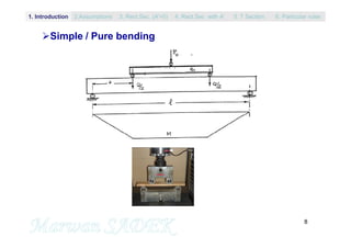
![45
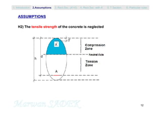
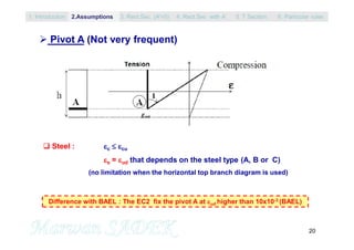
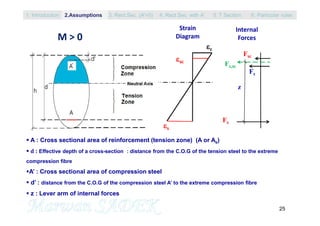
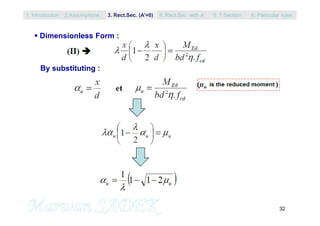
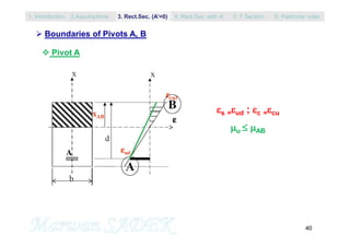
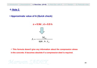
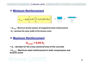
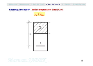
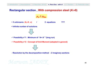
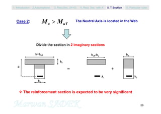
Minimum Reinforcement (to prevent brittle failure)
For rectangular section bh, the ultimate resistant bending moment of Non-
reinforced concrete :
MRc = (I/v) fctm = (b.h²/6) fctm
The minimum As,min section should resist the following moment
MRs = As,min fyk z
By considering MRc = MRs , and substituting z 0.9 d ; h d / 0.9
As,min = b.d.[fctm/(0.9 0.81 6)fyk] 0.23 b d fctm / fyk
L’EC2 replace the value of 0.23 by 0.26 and fix a lower limit of the quantity 0.26 fctm/fyk
with the value 0.0013
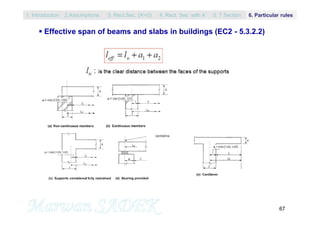
1. Introduction 3. Rect.Sec. (A’=0) 5. T Section2.Assumptions 4. Rect.Sec with A’ 6. Particular rules](https://image.slidesharecdn.com/rcs1-chapter5-170312083933/85/Rcs1-Chapter5-ULS-45-320.jpg)
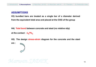
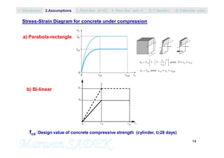
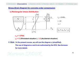
![50
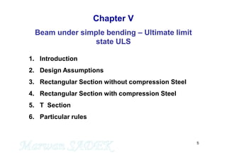
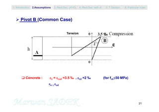
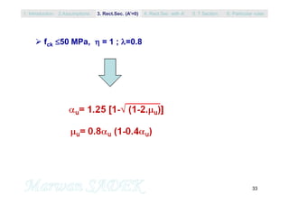
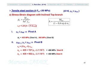
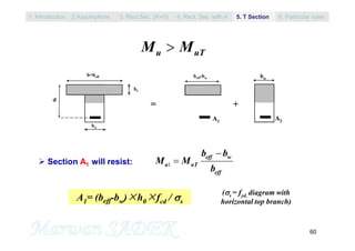
cu
s
sc
x=lim.d
d’
d
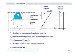
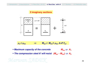
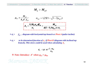
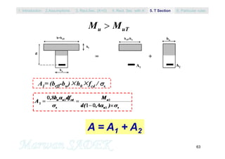
A1 = Mlim / (1 – 0.4.lim).d.fyd
A’ = (Med – Mlim) / [sc . (d-d’)]
sc = 3,5.10-3. (1-d’/xlim)
The value of sc is close to 3 °/°° (>se), in other terms sc=fyd when using the diagram
with horizontal top branch, and a value slightly great than fyd when using the diagram
with inclined top branch.
In general, we take a value sc=fyd .
A2 = A’. sc / s = A’. fyd / s
1. Introduction 3. Rect.Sec. (A’=0) 5. T Section2.Assumptions 4. Rect.Sec with A’ 6. Particular rules](https://image.slidesharecdn.com/rcs1-chapter5-170312083933/85/Rcs1-Chapter5-ULS-50-320.jpg)
![51
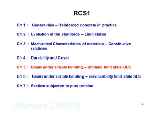
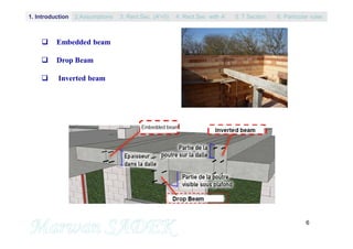
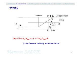
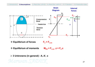
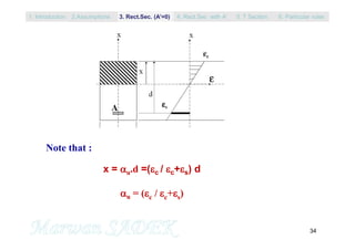
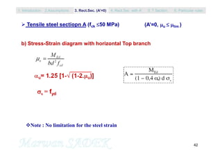
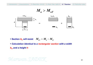
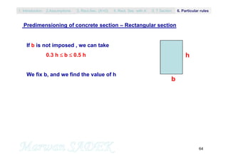
A1 = Mlim / [(1 – 0.4.lim).d.fyd]
A2 = A’. sc / s
A’ = (Med – Mlim) / [fyd . (d-d’)]
When using same types and grade for A and A’ sc = s = fyd
A2 = A’
A = A1 + A2
1. Introduction 3. Rect.Sec. (A’=0) 5. T Section2.Assumptions 4. Rect.Sec with A’ 6. Particular rules](https://image.slidesharecdn.com/rcs1-chapter5-170312083933/85/Rcs1-Chapter5-ULS-51-320.jpg)

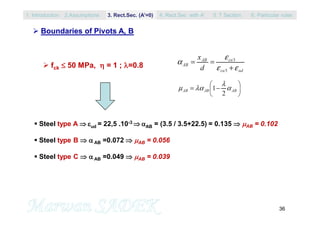
The document outlines the fundamentals of reinforced concrete structures, covering topics such as design assumptions, mechanical characteristics, durability, and various limit states for beams under simple bending. It references the evolution of standards and incorporates multiple sources, including the Eurocodes and previous French codes. Key elements discussed include stress-strain relationships, section analysis, and design considerations applicable to structural engineering practices.