
More Related Content
What's hot
What's hot (20)
Viewers also liked
Viewers also liked (20)
Similar to Navier stokes equation
Similar to Navier stokes equation (20)
Recently uploaded
Recently uploaded (20)
Navier stokes equation
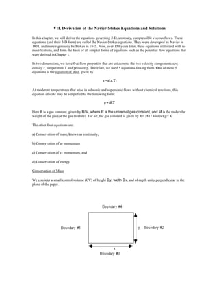
- 1. VII. Derivation of the Navier-Stokes Equations and Solutions In this chapter, we will derive the equations governing 2-D, unsteady, compressible viscous flows. These equations (and their 3-D form) are called the Navier-Stokes equations. They were developed by Navier in 1831, and more rigorously be Stokes in 1845. Now, over 150 years later, these equations still stand with no modifications, and form the basis of all simpler forms of equations such as the potential flow equations that were derived in Chapter I. In two dimensions, we have five flow properties that are unknowns: the two velocity components u,v; density r, temperature T and pressure p. Therefore, we need 5 equations linking them. One of these 5 equations is the equation of state, given by At moderate temperatures that arise in subsonic and supersonic flows without chemical reactions, this equation of state may be simplified to the following form: Here R is a gas constant, given by R/M, where R is the universal gas constant, and M is the molecular weight of the gas (or the gas mixture). For air, the gas constant is given by R= 2817 Joules/kg/° K. The other four equations are: a) Conservation of mass, known as continuity, b) Conservation of u- momentum c) Conservation of v- momentum, and d) Conservation of energy. Conservation of Mass We consider a small control volume (CV) of height Dy, width Dx, and of depth unity perpendicular to the plane of the paper.
- 2. The principle of conservation of mass states that "The rate at which mass increases within the control volume = The rate at which mass enters the control volume through its four boundaries" Let r be the average density of the fluid within the control volume. Then, Next, consider the rate at which mass enters through the four boundaries, one by one. Consider the boundary #1, first. We can assume that the above flux is computed at the center of face #1. We can consider the other three boundaries in a similar manner. The rate at which mass enters through faces 2,3 and 4 are, respectively (-ruDy)2 , (+(rvDx)3 and (-rvDx)4. Here the subscripts refer to the face. Summing up the contributions from the four faces, and equating the result to the time rate of change of mass within the CV, we get Now, consider the limits of the above equation as Dx and Dy goes to zero. From calculus, for any arbitrary function f(x,y), Applying the above limits, and bringing all the terms to the left hand side, we get The above equation, in vector form is given by:
- 3. The vector form is more useful than it would first appear. If we want to derive the continuity equation in another coordinate system such as the polar, cylindrical or spherical coordinate system, all we need to know is (a) look up the 'Del' operator in that system, (b) look up the rules for the dot product of 'Del' operator and a vector in that system, (c) perform the dot product. Conservation of u- Momentum Equation Before we can proceed any further, we need to get a firm understanding of terms such as viscosity, viscous stresses, conductivity, etc. Consider the left face of the control volume considered earlier. The air molecules to the left of this CV can interact with our CV in one of three ways: (i) organized motion from left to right. While the molecules are constantly moving about back and forth, over a small period of time, the majority of these molecules either enter the control volume (u >0) or leave the control volume. This "average" over a period of time is called the flow velocity component u, and is measured by probes such as LDVs and hot wires. (ii) Exchange of u- momentum between the molecules on the left and those on the right by collisions. In this case, there no net gain in mass, but there is a gain (or loss) in momentum. These collision effects may be averaged over a sufficiently small period of time, and may be viewed as a pressure force exerted by the fluid on the left on our CV. Again, only this average effect is felt or measured by pressure probes, and barometers. The individual collisions occur far too rapidly and far too frequently to be sensed by probes or measuring devices. (iii) _Exchange of u- and v- momentum by random linear motion of molecules jumping in and out of our control volume, across the face 1. In this case, all the molecules that jumped in also jump out over a sufficiently small time period. Thus, this random motion does not add mass to our control volume (and was not considered in our "continuity" equation). They however bring u- and v-momentum in or out (associated with their random motion). The time averages of these rates at which u- and v- momentum is brought into the CV across a face are called viscous forces. The forces per unit area are called viscous stresses. The viscous stresses that bring in/out u- momentum are called normal viscous stresses, while those that bring in v- momentum (by entering the face at an angle) are called tangential viscous stresses. By convention, pressure forces are considered positive, if they act towards the fluid element, or control volume. The normal viscous stresses (following solid mechanics conventions) are considered positive if they act away from the control volume, producing a tension.
- 4. These stresses (normal, and tangential or shear) are given the symbol t. They are identified by two subscripts. (i) The first subscript indicates the plane on which they act. For example, if a plane is normal to the x- axis, the first subscript will be x. (ii) The second subscript identifies the direction of the force associated with the force. For example, if a shear force is pointing in the y- direction, the second subscript will be y. Thus, viscous stress is a tensor quantity, and requires three pieces of information (its magnitude, its direction and the plane on which it acts) to completely specify it. This separates a tensor from a vector (magnitude and direction), and a scalar (magnitude only).
- 5. Newtonian Fluids Because our primary unknowns are the flow properties (u,v,p,r,T) there is a need to link the stresses t with these physical variables. In solid mechanics (Hooke's law) stress is set proportional to strain. This works for solids because a solid undergoes only a finite amount of deformation when a force or stress is applied to it. In fluid mechanics, this approach does not work because fluid continuously deforms when a shear stress is applied. It is this characteristic that distinguishes a fluid from a solid. Newton came up with the idea of requiring the stress t to be linearly proportional to the time rate at which strain occurs. Specifically he studied the following problem. There are two flat plates separated by a distance 'h'. The top plate is moved at a velocity V, while the bottom plate is held fixed. Newton postulated (since then experimentally verified) that the shear force or shear stress needed to deform the fluid was linearly proportional to the velocity gradient:
- 6. The proportionality factor turned out to be a constant at moderate temperatures, and was called the coefficient of viscosity, m. Furthermore, for this particular case, the velocity profile is linear, giving V/h = ∂u/∂y. Therefore, Newton postulated: Fluids that have a linear relationship between stress and strain rate are called Newtonian fluids. This is a property of the fluid, not the flow. Water and air are examples of Newtonian fluids, while blood is a non- Newtonian fluid. Stokes Hypothesis: Stokes extended Newton's idea from simple 1-D flows (where only one component of velocity is present) to multidimensional flows. here, the fluid element may experience a strain rate both due to gradients such as ∂u/∂y as well as ∂v/∂x. He developed the following relations, collectively known as Stokes relations. These expressions hold for 3-D flows. For 2-D flows, somewhat simpler expressions are obtained if we set w, the z- component of velocity, to zero, and if we set all derivatives with respect to z to be zero. The quantity m is called the molecular viscosity, and is a weak function of temperature. For air viscosity increases with temperature, because viscous effects are associated with random molecular motion. The coefficient l was chosen by Stokes so that the sum of the normal stresses txx, tyy and tzz are zero. Then The above equation, and the requirement that the three normal stresses add up to zero are called Stokes hypothesis. Returning Back to u- Momentum Equation....
- 7. We now return to the derivation of the u- momentum equation. This equation is a generalization of Newton's second law of motion, and may be verbally stated as: "The rate of change of u- momentum within a control volume is equal to the net rate at which u- momentum enters the control volume + Forces (pressure, viscous and body) acting on the control volume in the x- direction" As before we consider the control volume of height Dy and width Dx. We neglect body forces such as gravity, electrical and electromagnetic effects. Summing up these contributions, dividing through DxDy and taking the limits as Dx and Dy go to zero, we get:
- 8. Derivation of v- Momentum Equation: The v- momentum equation may be derived using a logic identical to that used above, and is left as an exercise to the student. The final form is: Derivation of the Energy Equation: The energy equation is a generalized form of the first law of Thermodynamics (that you studied in ME3322 and AE 3004). The only difference here is that we are studying an open system (i.e. control volume) that can gain and lose mass. The classical form studied in courses on thermodynamics is applicable only for closed systems - i.e. fixed collection of particles. The first law of Thermodynamics states that "(A) The rate at which the total (i.e. internal + kinetic) energy increases within a control volume is equal to (B) the rate at which total energy enters the control volume + (C) the rate at which work is done on the control volume boundary by surface forces + (D) the rate at which work is done on the CV by body forces + (E) the rate at which heat is added to the control volume at the surfaces by heat conduction + (F) the rate at which heat is released is added within the CV due to chemical reactions." In our derivation, we will neglect the term (D) which corresponds to the work done by the body forces (such as gravity, electrical and electromagnetic forces) and (F) which corresponds to chemical reactions. In some applications, e.g. modeling of weather, term D is important, while in others (e.g. modeling combustors) term F is important. We define the specific total energy (i.e. total energy per unit mass) E as In the above equation 'e' is specific internal energy. The word 'specific' means 'per unit mass'. Term A: Then, term A may be expressed as follows:
- 9. Term B: Term B involves mass entering and leaving the four boundaries of the CV, carrying with it, the total energy E. This term may be expressed as: As in the continuity equation, as Dx and Dy go to zero, the terms within the square brackets will go to -∂(ruE)/∂x and -∂(rvE)/∂y, respectively. Term C: At the surfaces of the control volume, there are pressure and viscous forces that do work on the fluid, as the fluid particles cross the boundary. For examples, on face #1, the pressure forces and viscous forces may be expressed as . The fluid velocity at this boundary is . The rate at which work is done by the surface forces acting on face #1 is, then, Summing up contributions from all the four faces, we get ,
- 10. Term D: The work done by body forces is neglected here. Term E: The heat conduction effects are associated with the random motion of gas molecules across the control volume. As they move in and out, they bring energy into and out of the control volume. When integrated over a small but finite period of time, a net exchange of heat energy occurs at the boundary, without any exchange in mass. Since this process is a random, chaotic process, it must somehow be empirically modeled. We adapt Fourier's law used to model conduction of heat through solids, which states "The rate at which heat flows across a surface of unit area is proportional to the negative of the temperature gradient normal to this surface". The constant of proportionality is called conductivity k, a property of the solid (or fluid, in the present context). Note that the heat flux is proportional to the negative of the gradient, because heat flows from hot to cold. We can sum up the heat conduction effects at all the four boundaries. The result is, Summing up all the terms A through E, and dropping the common factor DxDy that appears everywhere, we get the energy equation.
- 11. Prandtl Number: The coefficient of conductivity k is a property of the fluid, like the molecular viscosity. It is also a weak function of temperature and so is the molecular viscosity. Both these empirical coefficients are associated with transport of energy and momentum by random molecular motion. It follows that these two terms should be, somehow, related. Indeed, the following simple relationship exists. Here, Cp is the specific heat at constant pressure. The quantity Pr is called the Prandtl number, and is a property of the fluid. For air Pr is around 0.72 (close to unity). It is a measure of the ratio between the viscous effects and conduction effects. In some highly conductive, but only slightly viscous fluids such as mercury, Pr is very small. In other fluids such as honey which is highly viscous, but only slightly conductive, Pr is very high. Sutherland's Law: For air, the variation of viscosity (and hence conductivity) with temperature may be empirically described y the Sutherland's Law which states: where m0 denotes the viscosity at the reference temperature T0, and S1 is a constant. For air, S1 assumes the value 110 degrees kelvin. Summary The 2-D unsteady Navier-Stokes equations may be written in a number of forms. One common form of these equations is as follows: Continuity: u- Momentum:
- 12. v-Momentum: Energy Equation: Here. ρ= density; u,v = Cartesian Components of velocity along x,y axes; p = Pressure ; T = Temperature. Also, e = Specific Internal Energy = Internal energy per unit mass of the fluid = CvT , where Cv is the specific heat at constant volume. h0 = Specific Total Enthalpy = Total enthalpy per unit mass of the fluid = CpT+(u2+v2)/2 , where Cp is the specific heat at constant pressure. Finally, the viscous stresses are related to the velocity field by Stokes relations
- 13. The molecular viscosity m and conductivity k are properties of the fluid and are functions of temperature. These two quantities are related by the Prandtl number For air, the Prandtl number is around 0.72 at room temperatures. Simplified Form for Steady, 2-D Incompressible Flows: In steady, incompressible flows, we can drop the time derivatives because the flow is steady. The density may be also assumed constant. Then, the first three equations in the full Navier-Stokes equations set become: where n is called the kinematic viscosity=µ/ρ Nondimensionalization of the Viscous Flow Equations Consider the 2-D viscous flow past an airfoil shown below:
- 14. At first glance it appears that such a flow will depend on a large number of parameters such as (a) airfoil shape, including its chord c ,(b) its angle of attack, (c) the freestream temperature T∞ (d) the freestream density r∞ , (e) the freestream velocity V∞, (f) the freestream viscosity m∞, (g) the freestream conductivity k∞, and so on. We wish to know if these large number of physical and geometric parameters can be grouped into a handful of parameters that can be systematically varied to study their effect on the flow. There are two common ways of identifying these parameters: (i) Dimensional analysis: Here we attempt to combine the parameters listed about to arrive at a nondimensional form. For example, after some trial and error, we can show that the quantity r∞Vc/m∞ is a nondimensional quantity. Intuition and experience are needed to realize that this nondimensional parameter, called Reynolds number, is also a useful physical parameter. Dimensional analysis will also produce combinations such as . This parameter, while nondimensional, is not a significant parameter in incompressible flows, as experience shows. (ii) Nondimensionalization of Governing Equations: This approach provides a formal manner by which nondimensional parameters of physical significance may be uncovered. This approach is usually used in combination with the dimensional analysis shown above. To illustrate how this approach works, let us consider the 2- flow over an airfoil shown above. Let us introduce nondimensional quantities identified with a prime (') as follows: When these nondimensional quantities are used to replace the corresponding physical quantities in the continuity equation the following form results: This form looks identical to the dimensional form given in Handout #1, and no new nondimensional parameter emerges. If we repeat this process with the u- momentum equation, and replace terms such as txy and p with terms such as
- 15. we get, after some minor algebra: If we repeat this process with the v- momentum equation, again the Reynolds number emerges as the nondimensional parameter. Consider two different flows over the same airfoil, but of different chord. The present normalization shows that these two flows are governed by the same nondimensional form of the governing equations, and will result in the same nondimensional flow quantities such as u', v' etc. if the flows are geometrically similar (same airfoil shape, same a), and dynamically similar (same Reynolds number). The parameter Reynolds number may also be interpreted in another way. Consider a typical inviscid term such as p appearing on the left side of the u- momentum equation. This "inertial" force term is roughly of order . Consider a viscous stress term such as txy. This term is of order . Then, Reynolds number is a measure of the ratio between the inertial forces and viscous forces acting on a fluid element. If this number is large, then inertial forces dominate over viscous forces and vice versa. In practical aeronautical applications, the Reynolds number is invariably large. For example, the airfoil over a helicopter rotor blade operates at a Reynolds number of 3 to 5 Million, while the airfoil in the Root section of a modern transport aircraft operates at a Reynolds number of 30 to 50 Million. In such flows, viscous forces are small and may be neglected over most of the flow, except in very small regions called boundary layers over the airfoil. Nondimensionalization of the Energy Equation: If we nondimensionalize the energy equation by the same principles, we get, in addition to the Reynolds number, the parameter . This parameter occurs due to the presence of the heat conduction terms and viscous stress work terms in the energy equation. This parameter is called the Prandtl number, and is a property of the fluid. For air, Prandtl number is around 0.72. In compressible flows, the quantity is a nontrivial quanity and must be prescribed. Using equation of state, the definition of the speed of sound and the definition of Mach number, we can relate this quantity to the Mach number and the ratio of specific heats, g.
- 16. Thus, in compressible flows, two flows are identical if they are geometrically similar and if Reynolds number, Mach number, Prandtl number and ratio of specific heats all match. In incompressible flows, this quantity is not a significant parameter. As hydraulics engineers will attest, raising the static pressure at some point in the flow simply raises the pressure level everywhere by the same constant level, and does not alter the flow behavior. Some Exact Solutions of the Navier-Stokes Equations We next turn our attention to the exact solutions of incompressible Navier-Stokes equations. Even though these equations were derived over a century ago, only a handful of exact solutions exist for some highly simplified situations. This is because of the nonlinear nature of these equations. The governing equations are: In the above equations, we have assumed the conductivity k and viscosity m to be constant. We will further restrict ourselves to steady flows (∂/∂t = 0) , and incompressible flows (r = constant). The above form of equations apply only to 2-D planar flows. Similar forms of Navier-Stokes equations exist in other coordinate systems such as the cylindrical, polar and spherical coordinate systems. Parallel Flows The first class of flows to be considered is the flow between (or within) infinitely long parallel plates, and infinitely long tubes.
- 17. In such flows, it is reasonable to assume that the flow behavior will be independent of the x- location. That is, x-derivatives of all flow properties such as ∂u/∂x, ∂v/∂x, ∂T/∂x etc. vanish. The pressure derivative ∂p/∂x is assumed to be a constant, required to drive the flow. In such as situation, continuity equation becomes Setting ∂u/∂x=0 yields ∂v/∂y = 0 or ∂(rv)/∂r=0. The assumption ∂v/∂x=0 implies that the velocity component v is not a function of x. Thus, continuity yields v = constant, for our flows. Since the boundary condition requires v to be zero at the walls of our parallel plates, and at the walls of the tube, continuity + boundary conditions together yield In other words, the flow only has a u- component and is parallel to the x- axis. For this reason, the first class of flows we study are called parallel flows. Exact Solution # 1: Planar Couette Flow: In 1890 Couette performed experimental studies of flow between two concentric cylinders, where one of the cylinder is fixed, the other is spinning. This situation is similar to what happens in a ball bearing. here we study the 2-D analog of flow between two parallel plates. One of the plate is held fixed, while the other one is moving at a velocity V. The plates are separated by a distance h. A constant pressure gradient dp/dx is applied to this flow.
- 18. For this case, the u- momentum equation yields Setting the x- derivatives to zero, and requiring v to ve zero, the above equation may be simplified to yield Notice that we have begun to replace partial derivatives with respect to y with ordinary derivatives, because flow properties are only functions of y. Integrating the above equation twice, we get: where A and B are constants of integration. These may be evaluated by requiring u=0 at y=0 and u= V at y=h. Two special situations are of interest. In the first case, the pressure gradient dp/dx=0 is zero, and the flow motion is brought about by the motion of the top plate at the constant velocity V. In that case, the velocity profile is linear, giving
- 19. u(y) = V y/h In the second situation, both the plates are at rest and V=0. the fluid is motion is caused by the application of pressure gradient dp/dx. In this case, the velocity profile is a parabola, given by The shear stress txy(i.e. the force per unit area exerted by the fluid on the flat plates, and vice versa) may be computed from Stokes' relations. For example, for the case where dp/dx=0, we get The non-dimensional "skin friction" coefficient Cf is then computed as Temperature Distribution for Planar Couette Flow: The energy equation, which is part of the Navier-Stokes equations is usually not solved in incompressible flow applications, unless we are interested in a heat transfer application. Let us consider the situation where dp/dx=0, the top plate is moving at the velocity V, and the pressure gradient dp/dx=0. Let the bottom and top plates be at two different temperatures T1 and T2 respectively. In this case, we can easily solve for the temperature distribution in the fluid between the plates, and compute the rate at which heat is transferred from the hot plate to the cold plate, as follows. The energy equation for this case is (Verify for yourself, starting with the form given in Handout #1):
- 20. For our parallel flow, we can set ∂/∂x =0 and v = 0. For the case where dp/dx=0, the velocity profile is linear, as derived earlier. Then, When these expressions are substituted into the energy equation, and when all x-derivatives are set to zero, and when v is set to zero, the following form results. Integrating the above equation twice, we get where C and D are constants of integration. These constants may be found by applying the boundary condition T= T1 at y=0, and T = T2 at y= h. The final form is The first two terms in the above expression are linear in y, and model the effect of conduction on the temperature distribution. The third term models the effect of heat geeration due to viscous work. Since m is small, this term is likely to be of significance only in high speed flows.