Download as PDF, PPTX


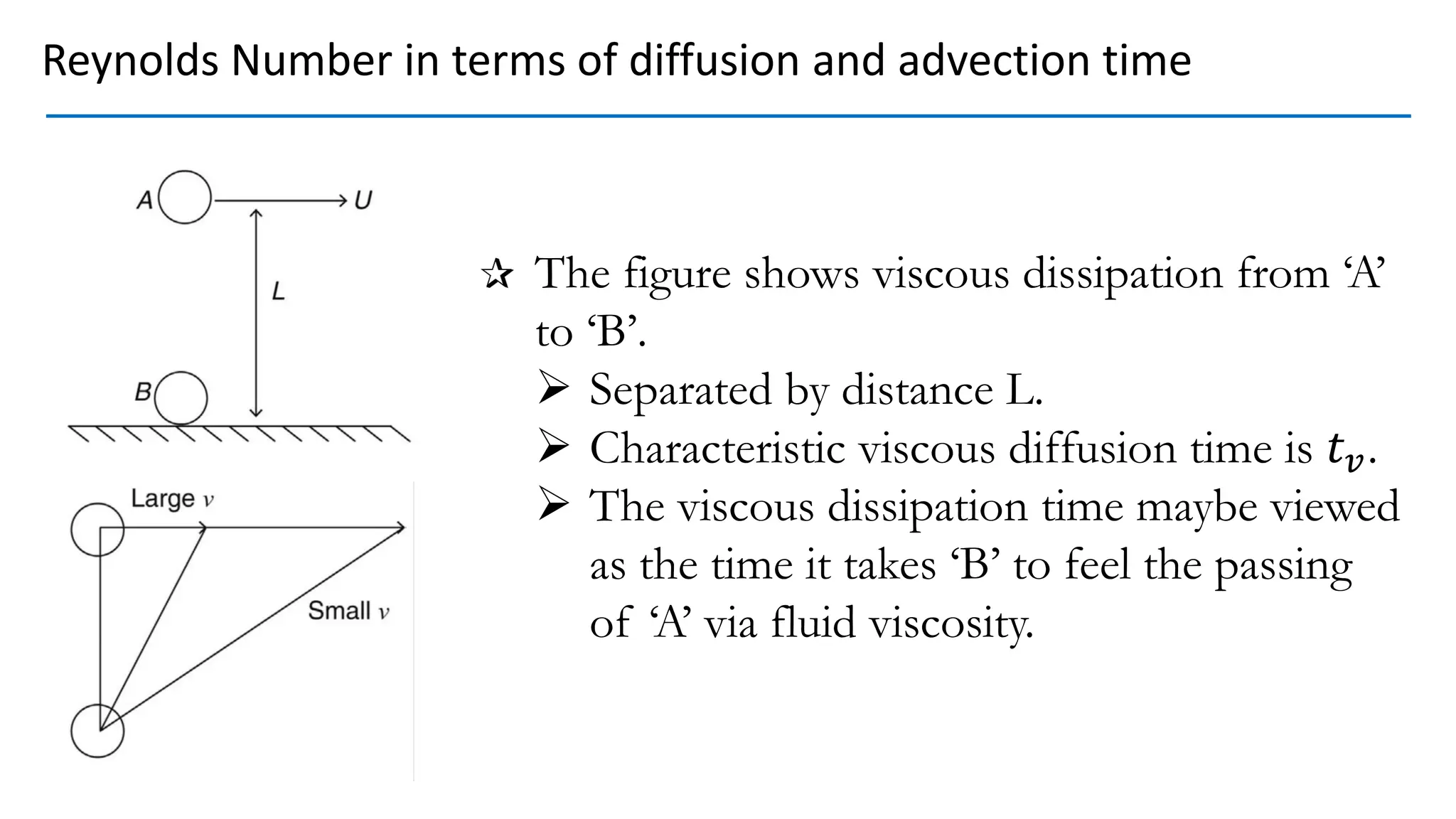

![Hence dimensionally the characteristic viscous diffusion time
which is required for momentum to diffuse a distance ‘𝐿’ due to
viscosity is
𝑡𝑣 =
𝐿2
𝜈
; [ Τ
𝑚2 Τ
𝑚2
𝑠 = 𝑠]
For a body of length ‘𝐿’ in a flow field with a mean velocity ‘𝑈’.
A characteristic(overall) advection time scale 𝑡𝑎 signifies the
duration over which the fluid element is of significance to the
body and vice-versa.
𝐴𝑑𝑣𝑒𝑐𝑡𝑖𝑜𝑛 𝑇𝑖𝑚𝑒 𝑡𝑎 =
𝐿
𝑈
Advection time is the time that is required by a fluid element to
pass a body of length ‘𝐿’.
Reynolds Number in terms of diffusion and advection time](https://image.slidesharecdn.com/turbulencescales-210422004612/75/Scales-in-Turbulent-Flow-9-2048.jpg)


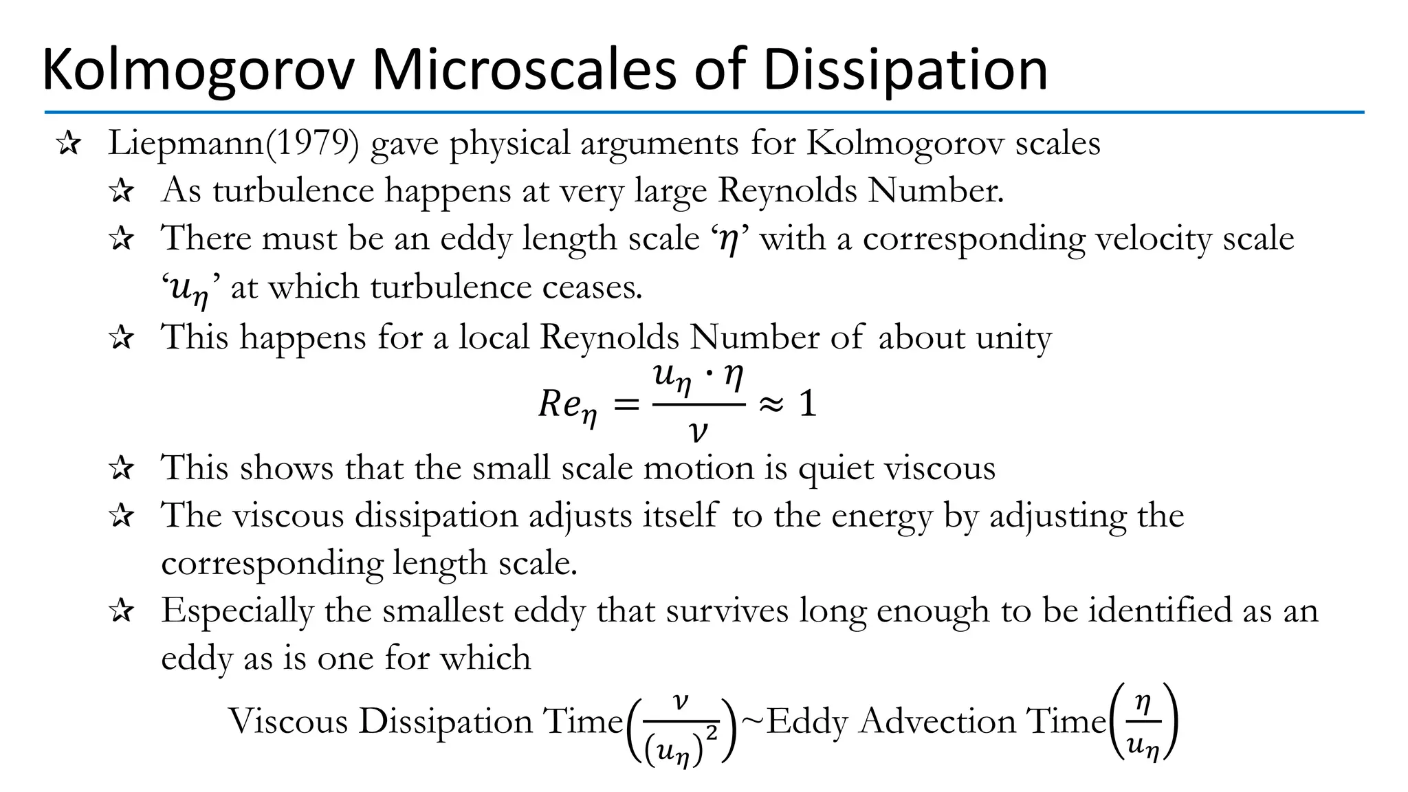
![Combining these ideas Kolmogorov proposed that length, velocity and time-
scales of dissipation must be function of dissipation rate and viscosity only.
𝜂 = 𝑓 𝜀, 𝜈
𝑢𝜂 = 𝑓 𝜀, 𝜈
𝑡𝜂 = 𝑓(𝜀, 𝜈)
Note that is hypothesis is only valid when:
𝑆𝑖𝑧𝑒 𝑜𝑓 𝑑𝑖𝑠𝑠𝑖𝑝𝑎𝑡𝑖𝑜𝑛 𝐸𝑑𝑑𝑦 ≪ [𝑆𝑖𝑧𝑒 𝑜𝑓 𝑃𝑟𝑜𝑑𝑢𝑐𝑡𝑖𝑜𝑛 𝐸𝑑𝑑𝑦]
If the above is not the case, then eddies maybe simultaneously involved in both
production and dissipation.
Further, the length-scale of the eddies(i.e. dissipating and producing) will be
influenced by mean shear in addition to dissipation rate(𝜀) and viscosity (𝜈).
The above case will not be further explored as we are dealing with fully
developed turbulent flows, where Kolmogorov's hypothesis is valid.
Kolmogorov Microscales of Dissipation](https://image.slidesharecdn.com/turbulencescales-210422004612/75/Scales-in-Turbulent-Flow-33-2048.jpg)
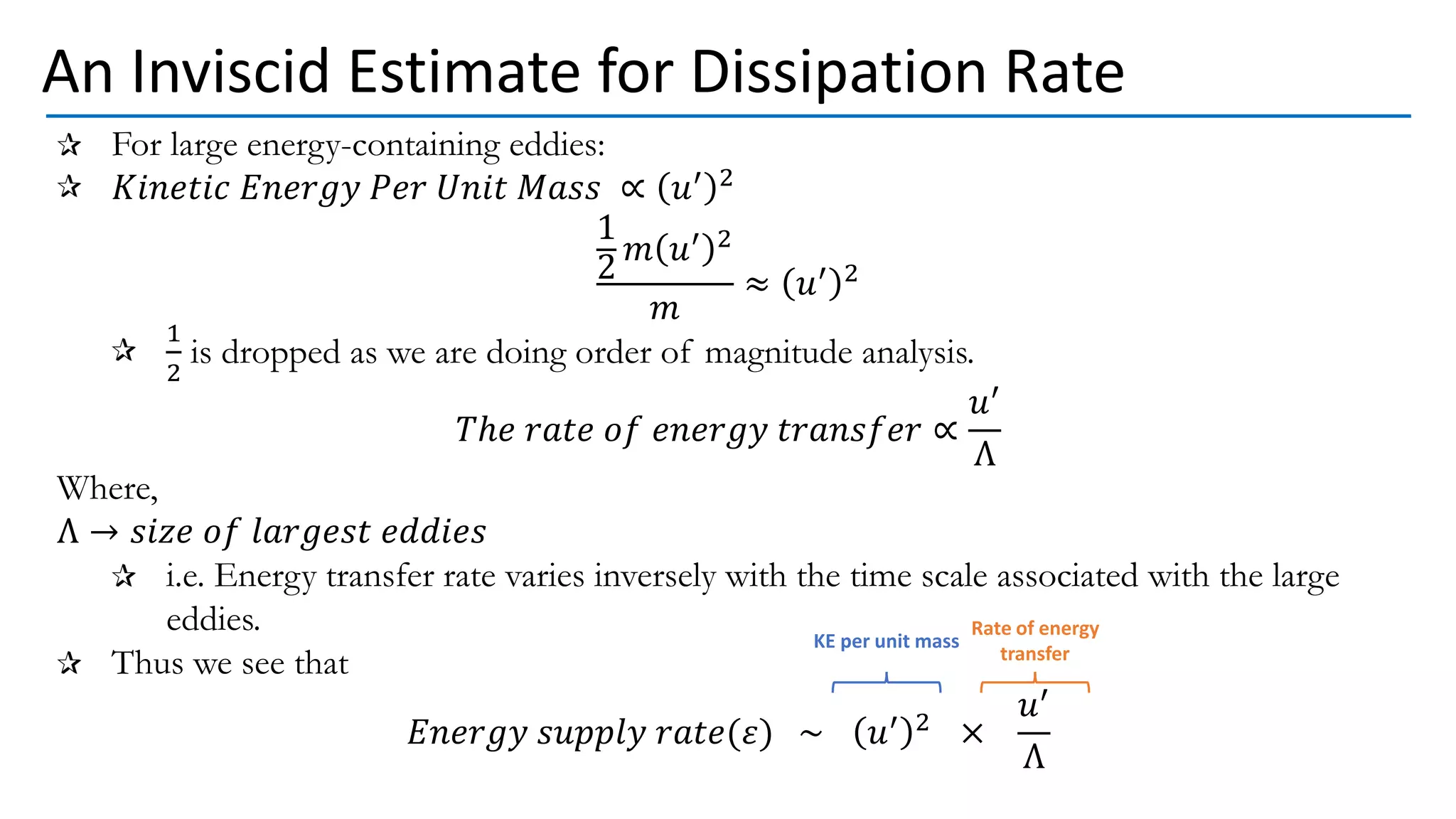
![From dimensional analysis:
𝜂 𝑚 ~𝜀𝑎[ Τ
𝑚2 𝑠3]𝜈𝑏[ Τ
𝑚2 𝑠]
Where,
𝑎 = − Τ
1
4 & 𝑏 = Τ
3
4
Further, the dimensional analysis yields
𝑆𝑚𝑎𝑙𝑙 𝑒𝑑𝑑𝑦 𝑙𝑒𝑛𝑔𝑡ℎ − 𝑠𝑐𝑎𝑙𝑒 𝜂 =
𝜈3
𝜀
ൗ
1
4
𝑆𝑚𝑎𝑙𝑙 𝑒𝑑𝑑𝑦 𝑣𝑒𝑙𝑜𝑐𝑖𝑡𝑦 − 𝑠𝑐𝑎𝑙𝑒 𝑢𝜂 = 𝜀𝜈 ൗ
1
4
𝑆𝑚𝑎𝑙𝑙 𝑒𝑑𝑑𝑦 𝑡𝑖𝑚𝑒 − 𝑠𝑐𝑎𝑙𝑒 𝑡𝜂 =
𝜈
𝜀
ൗ
1
2
Kolmogorov Microscales of Dissipation](https://image.slidesharecdn.com/turbulencescales-210422004612/75/Scales-in-Turbulent-Flow-34-2048.jpg)
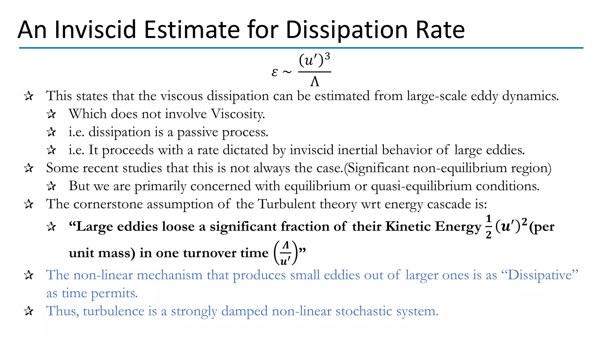
![The above suggest that:
“The eddying fluid motion dissipates completely, transforming all it’s Kinetic Energy via viscosity
into heat within one rotation”
Thus,
Energy dissipation is completely viscous.
All the energy produced from the mean flow is dissipated by small scales.
The overall dissipation rate(𝜀) is equal to the small scale rate
𝜀 =
𝜈 𝑢𝜂
2
𝜂2
Τ
𝑚2
𝑠3
~[ Τ
𝑊 𝑘𝑔]
Solving the previous two equation yields the Kolmogorov length scales 𝜂 and 𝑢𝜂.
𝜈 ↑ → 𝜀 ↑
𝑢𝜂(↑) → 𝑆ℎ𝑒𝑎𝑟(↑) → 𝜀(↑)
𝜂 ↑ → 𝑉𝑒𝑙𝑜𝑐𝑖𝑡𝑦 𝐺𝑟𝑎𝑑𝑖𝑒𝑛𝑡(↓) → 𝜀(↓)
Kolmogorov Microscales of Dissipation](https://image.slidesharecdn.com/turbulencescales-210422004612/75/Scales-in-Turbulent-Flow-36-2048.jpg)
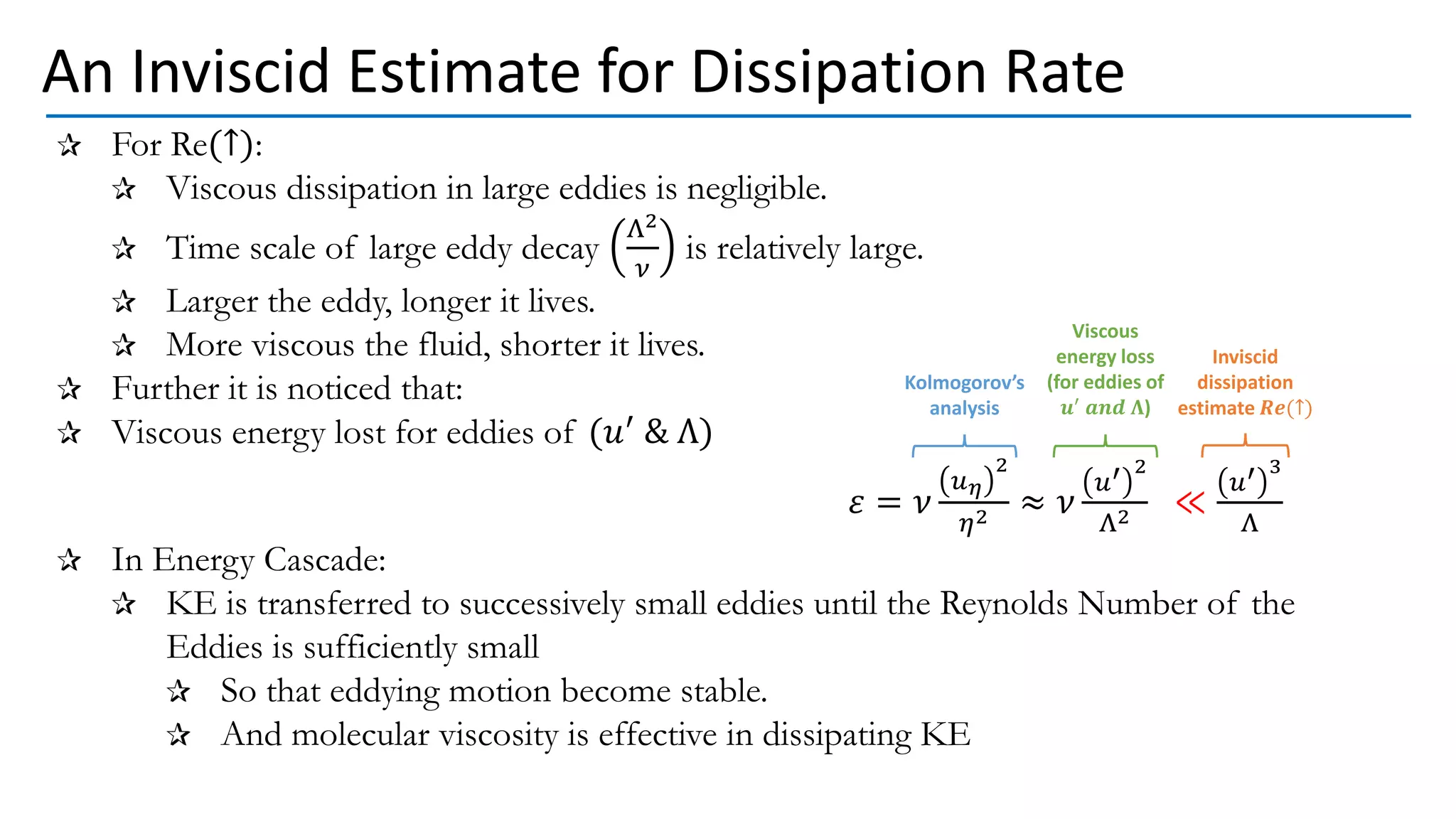
![Considering a mixing process where the fluid
involved has the following properties:
Kinematic Viscosity 𝜈 = 10−3 Τ
𝑚 𝑠
Density 𝜌 = 1000 Τ
𝑘𝑔 𝑚3
Suppose a 20 𝑊att electric mixer is used to mix a
1L mixture.
At equilibrium condition
𝐷𝑖𝑠𝑠𝑖𝑝𝑎𝑡𝑖𝑛𝑔 𝑝𝑜𝑤𝑒𝑟 𝜀 = 𝑃𝑜𝑤𝑒𝑟 𝐼𝑛𝑝𝑢𝑡 𝑃𝑖𝑛
𝜀 =
20[𝑊]
1000[ Τ
𝑘𝑔 𝑚3] × 0.001[𝑚3]
= 20 Τ
𝑊 𝑘𝑔
Kolmogorov Microscales of Dissipation
Kolmogorov and larger scales in a mixing process.](https://image.slidesharecdn.com/turbulencescales-210422004612/75/Scales-in-Turbulent-Flow-37-2048.jpg)


![Now taking look at vorticity [𝑠−1].
The small-large scale vorticity ratio is
𝑓𝜂
𝑓Λ
~
𝑡Λ
𝑡𝜂
~
𝜈
𝑢′Λ
1
2
= 𝑅𝑒
1
2
This shows that vorticity of smaller-scale eddies is much greater than, that associated with
large-scale eddies.
Thus, small-scale eddies rather than large scale eddies are used for modelling turbulence via
vorticity dynamics.
On the other hand, if we look at the corresponding distribution in the Turbulent Kinetic
Energy.
Mass of Kolmogorov eddy → 𝑚𝜂 ≈ 𝜌𝜂3
Mass of large eddy → 𝑚Λ ≈ 𝜌Λ3
𝑚Λ ≫ 𝑚𝜂
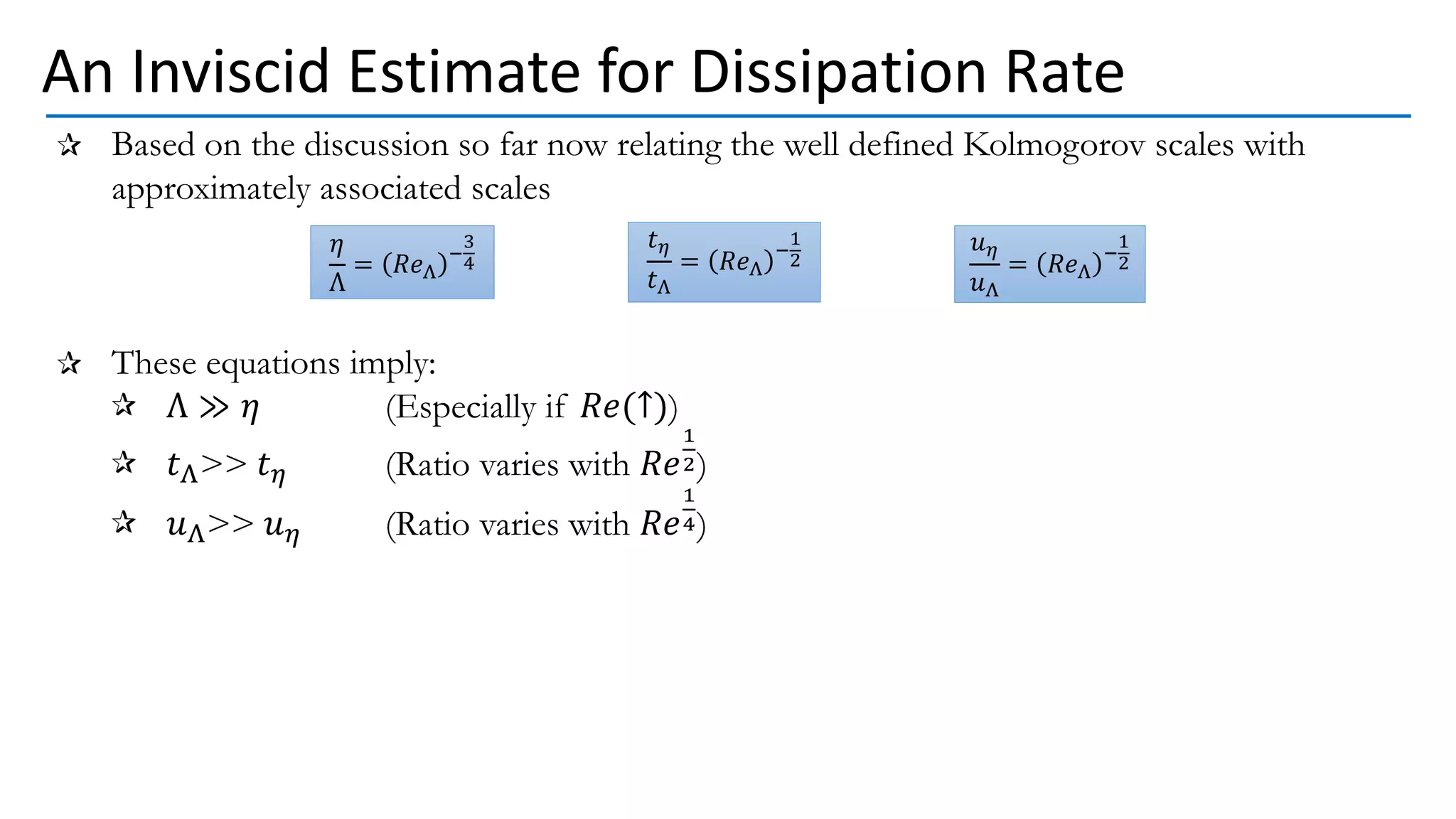
An Inviscid Estimate for Dissipation Rate](https://image.slidesharecdn.com/turbulencescales-210422004612/75/Scales-in-Turbulent-Flow-47-2048.jpg)


![In absence of [Pressure and Turbulent Diffusion] & [Viscous Work] we are
left with
𝐷
𝐷𝑡
𝑞′ 2
2
= 𝑃𝑟𝑜𝑑𝑢𝑐𝑡𝑖𝑜𝑛 −
𝑉𝑖𝑠𝑐𝑜𝑢𝑠
𝐷𝑖𝑠𝑠𝑖𝑝𝑎𝑡𝑖𝑜𝑛
The production TKE production rate (𝑃𝑡𝑢𝑟𝑏) & TKE dissipation rate 𝜀 .
𝑃𝑡𝑢𝑟𝑏 = −𝑢𝑖𝑢𝑗
𝜕𝑢𝑖
𝜕𝑥𝑗
[m2/s3] 𝜀 = 2𝜈𝑆𝑖𝑗
𝜕𝑢𝑖
𝜕𝑥𝑗
[m2/s3]
𝜀 = 2𝜈
1
2
𝜕𝑢𝑖
𝜕𝑥𝑗
+
𝜕𝑢𝑗
𝜕𝑥𝑖
𝜕𝑢𝑖
𝜕𝑥𝑗
; 𝑆𝑖𝑗 =
1
2
𝜕𝑢𝑖
𝜕𝑥𝑗
+
𝜕𝑢𝑗
𝜕𝑥𝑖
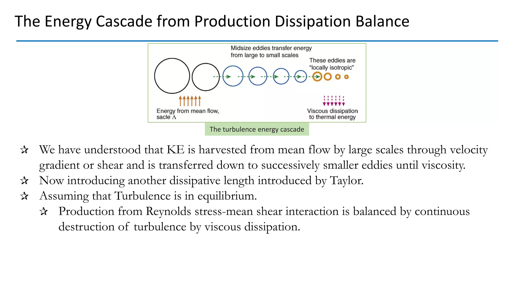
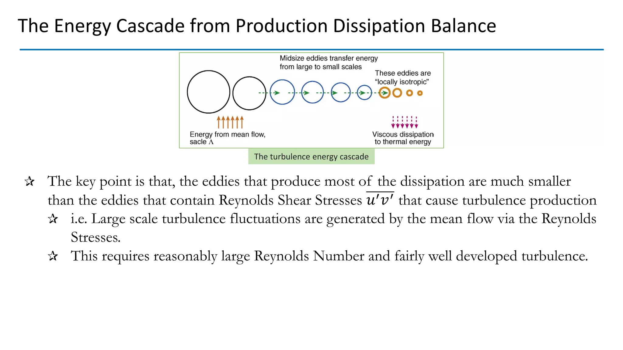
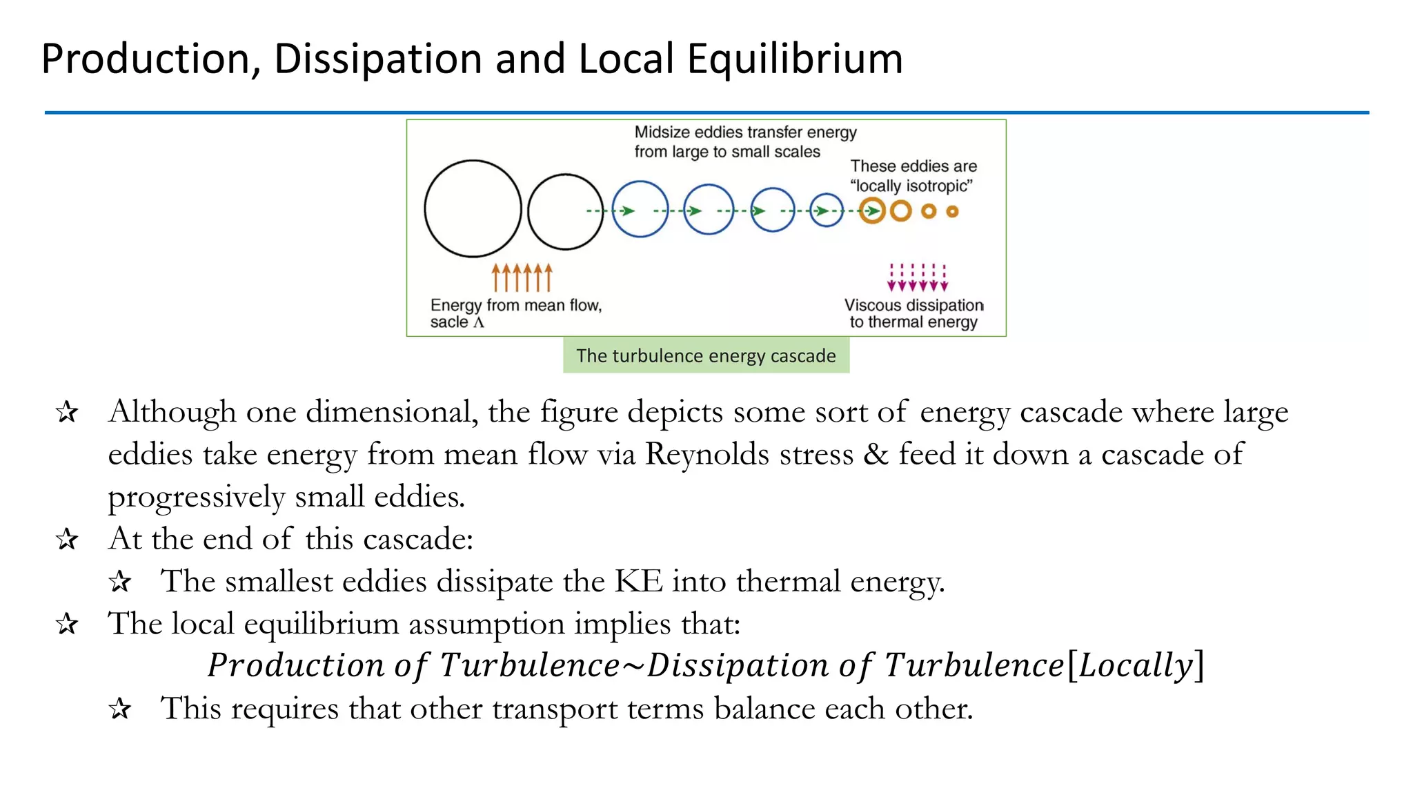
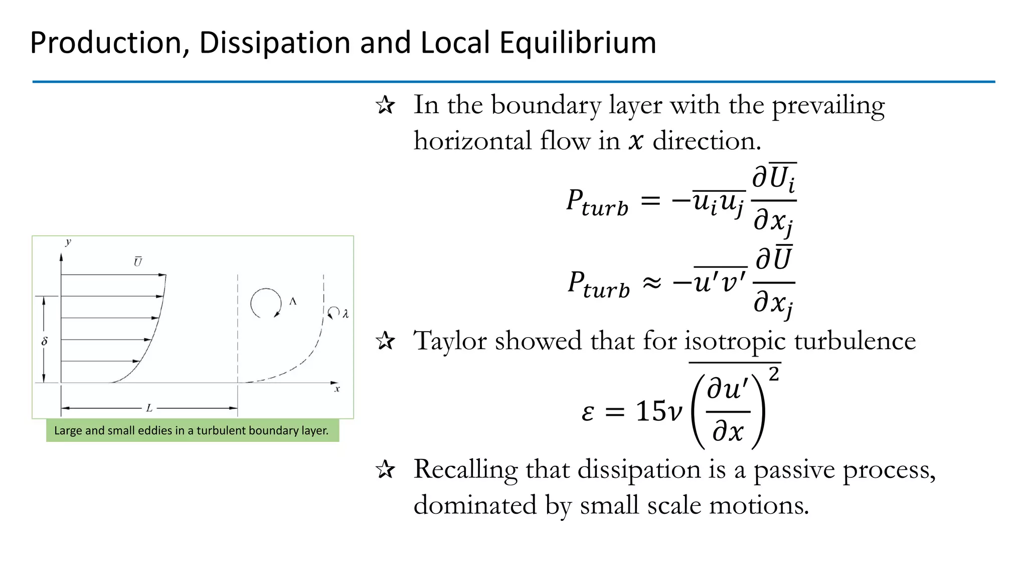
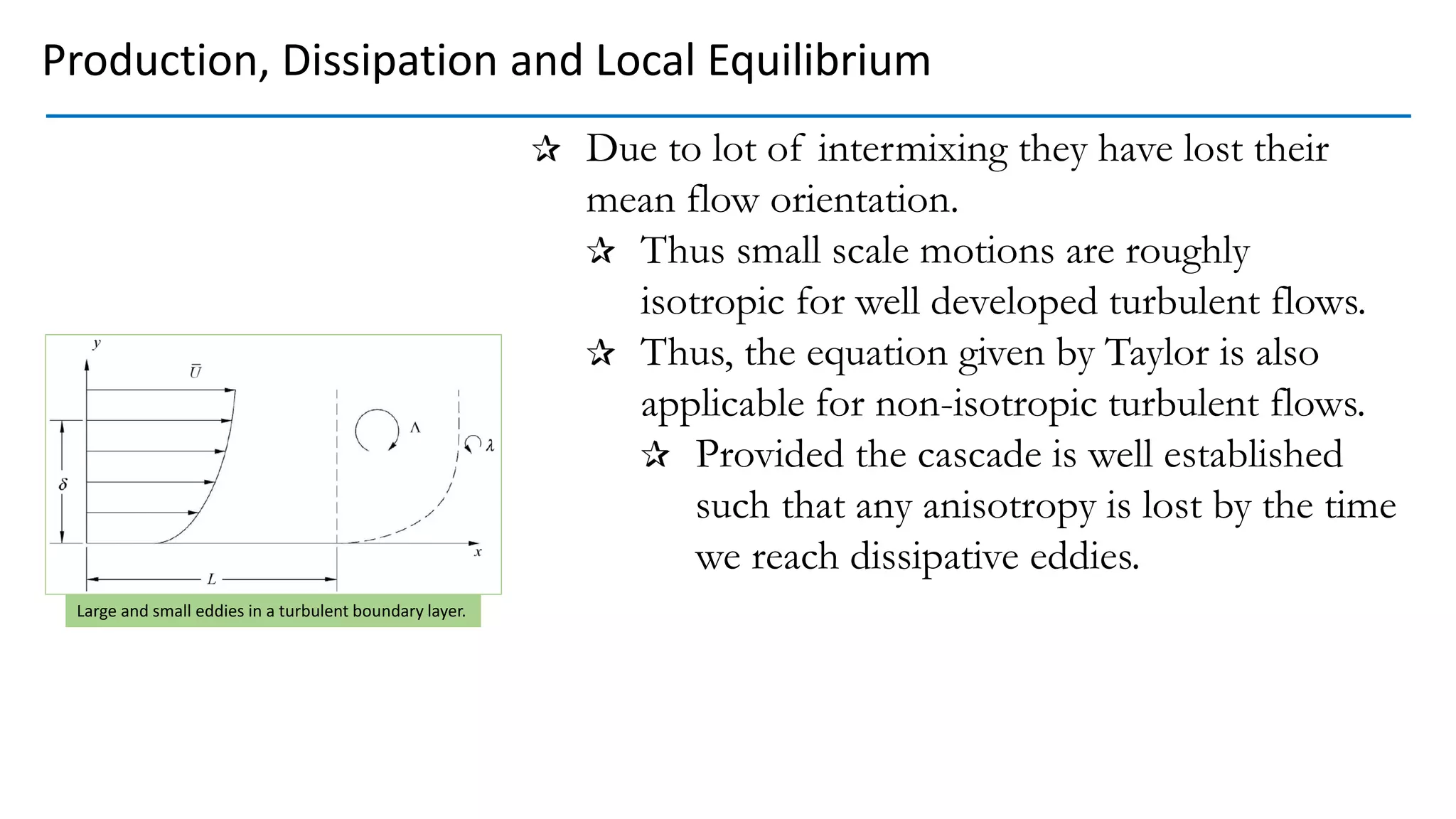
Production, Dissipation and Local Equilibrium
The turbulence energy cascade](https://image.slidesharecdn.com/turbulencescales-210422004612/75/Scales-in-Turbulent-Flow-54-2048.jpg)


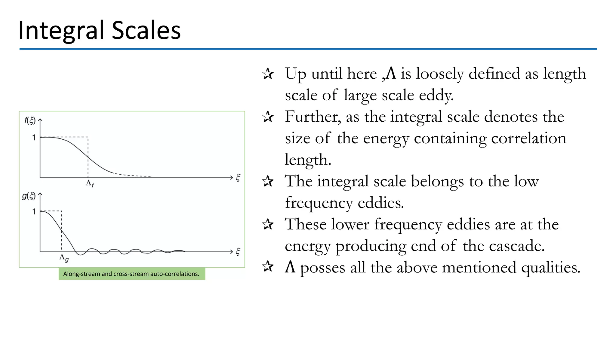


![Turbulent Kinetic Energy Spectrum
For well developed turbulence where Λ ≫ 𝜆,
we have
𝜀~
(𝑘𝑒)
3
2
Λ
[Taylor(1935)]
Which means
𝑘𝑒~(𝜀Λ)
2
3
As shown in the figure, for well developed
turbulence, there is a range of wavenumbers
over which neither production nor dissipation
is dominant.
i.e. inertial transfer of kinetic Energy is the
premiant player.
Orificed, perforated plate-generated streamwise
turbulence velocity spectra at U = 10.8 m/s.](https://image.slidesharecdn.com/turbulencescales-210422004612/75/Scales-in-Turbulent-Flow-80-2048.jpg)


This document discusses turbulent fluid flow and the scales involved. It states that fully developed turbulent flow involves a cascade from the largest eddies created by mean flow instabilities down to progressively smaller eddies. As eddy sizes decrease, dissipation and velocity gradients increase until energy is dissipated into heat at the smallest, viscous scales. The Reynolds number, which represents the ratio of inertial to viscous forces, is also derived and shown to relate the advection and diffusion time scales. Boundary layers in both laminar and turbulent flow are examined in terms of how viscosity affects fluid behavior at different length scales.