- The document discusses asymptotic analysis and Big-O, Big-Omega, and Big-Theta notation for analyzing the runtime complexity of algorithms. - It provides examples of using these notations to classify functions as upper or lower bounds of other functions, and explains how to determine if a function is O(g(n)), Ω(g(n)), or Θ(g(n)). - It also introduces little-o and little-omega notations for strict asymptotic bounds, and discusses properties and caveats of asymptotic analysis.

1. Data Structures and Algorithms with Java
Asymptotic Analysis Crash Course Review
CIS 121
Fall 2015

2. 1 Introduction and Intuition
In class, you have started to discuss tilde notation as a method of classifying functions and algorithms. Now
that you are more accustomed with this material, we introduce the more commonly used methods of runtime
analysis: Big-Oh and more generally, the Bachmann-Landau/asymptotic family of notations.
Before we get into the nitty-gritty, let’s look at a sample of code and analyze its runtime complexity first.
1 public void foo(int n) {
2 for (int i = 0; i < n; i++) {
3 System.out.println(i);
4 }
5 }
Simply by looking at this, you could probably guess that foo(n) runs in linear time (with respect to the
input size n). For the sake of being precise, let’s go a bit deeper. We let T(n) count the total number of
instructions computed with respect to n, i.e. the ”cost” of running the program. First, we count separately
the cost of all of the operations in foo(n).
operation cost times
variable declaration c1 1
less than compare c2 n + 1
increment c3 n
print c4 n
We use ci to denote a constant amount of work. Therefore, our T(n) is,
T(n) = c1 + (n + 1)c2 + nc3 + nc4
= (c1 + c2) + (c2 + c3 + c4)n
Our T(n) can thus be written in the form an + b, where a, b are constants. Thus, the amount of work
done is linear.
Still, it is pretty messy to consider all of these different constants. How would we even define ci? The
time cost of all of these operations varies widely across machines. With this in mind, we make a simplifying
abstraction: we are interested in the rate of growth, or order of growth, of the running time.
We therefore only consider the leading term of the formula for T(n), i.e. an, since the lower-order con-
stant term is relatively insignificant for large n. In fact, we even ignore the leading term’s coefficient a, since
constant factors are less significant than the rate of growth in determining computational efficiency!
We write that foo(n) runs in Θ(n) time (pronounced Theta of n). We use Θ-notation informally here
and will define it later.
For another example, suppose that T(n) = 1
1000 n3
− 100n2
+ 100n + 3. We can simply write that
T(n) = Θ(n3
).
We consider an algorithm as more efficient than another if the (worst-case) running-time has a lower
order of growth. You might say that an algorithm that runs in T(n) = n3
time might take less time than
one that runs in T (n) = 100n2
for small n, but for sufficiently large n, i.e. n > 100, the T (n) algorithm
will run more quickly than T(n).
2

3. Figure 1: *
100n2
vs. n3
2 Asymptotic Notation and Big-Oh
While asymptotic notation is primarily used to describe the running times of algorithms, it actually applies
to functions. When we were saying above that foo(n) ran in Θ(n) time, we really meant that T(n) = an+b
was Θ(n). For the next couple of sections, we’ll look at how asymptotic notation applies to functions before
going back to code.
Before we dive back into Big-Θ notation, let’s detour into a simpler and more well-known form of asymp-
totic notation, Big-Oh. We define Big-Oh notation as follows,
Big-Oh Notation
Definition. f(n) ∈ O(g(n)) if there exist positive constants n0 and c0 s.t. f(i) ≤ cg(i) for all i ≥ n0.
Simplified: If f(n) is in O(g(n)), g(n) is an asymptotic upper bound for f(n).
This can be somewhat daunting, but let’s look at what this says. A function f(n) is in the set of functions
O(g(n)) if g(n) is a loose upper bound for f(n).
You should understand that Big-Oh notation indicates a set of functions, but often-times we will switch
out ∈ for = to simplify things.
Example 2.1:
Let’s consider the functions f(n) = n, g(n) = 2n, h(n) = n2
.
Which functions are Big-Oh of each other?
We show that f(n) = O(g(n)).
n ≤ c · 2n
1
2
≤ c
Picking any c ≥ 1
2 will suffice, and picking any n0 > 0 will also work. Note that to prove Big-Oh
relations, you MUST pick a valid c and n0.
g(n) = O(f(n))
2n ≤ cn
2 ≤ c
3

4. Figure 2: *
n = O(n), n = O(n2
)
Picking any c ≥ 2 works, and picking any n0 > 0 satisfies the above relation.
So how can f(n) = O(g(n) and g(n) = O(f(n))? Recall that we defined Big-Oh relations as a loose
upper bound, so this should be very plausible.
Now let’s consider f(n) and h(n). f(n) = O(h(n)).
n ≤ cn2
We don’t really have to do much work here. Let us pick n0 = 1 and c = 1. It remains obvious that
n ≤ n2
for all n ≥ 1.
Then, is h(n) = O(f(n))? Clearly not! There is no c and n0 for which n2
≤ cn for all n ≥ n0. Therefore,
h(n) is what we call a strict upper bound for f(n). To describe a strict upper bound, we will later introduce
o-notation (little-oh).
Example 2.2:
Given f(n) = log n and g(n) =
√
n, show that f(n) ∈ O(g(n)).
log n ≤ c
√
n
log
√
n
2
≤ c
√
n
2 log
√
n ≤ c
√
n
At this point we can pick c = 2 and n0 = 1. It is evident that for these values, the RHS will always grow
faster than the LHS, due to a logarithmic difference in the order of growths.
4

5. Figure 3: *
log n vs. 2
√
n
Picking c and n0
From the examples shown above, you may have observed that c and n0 are chosen rather arbitrarily in the
Big-Oh proofs. There is no deterministic approach to picking c or n0 first. Sometimes, you may just have
to experiment and try picking multiple values for each before getting things to work out!
3 Big-Omega Notation
Up until this point we have only examined asymptotic upper bounds with Big-Oh. Let’s now flip the scales
and look at asymptotic lower bounds! We define Big-Ω as follows,
Big-Omega Notation
Definition. f(n) ∈ Ω(g(n)) if there exist positive constants n0 and c s.t. f(i) ≥ cg(i) for all i ≥ n0.
Simplified: If f(n) is Ω(g(n)), g(n) is an asymptotic lower bound for f(n).
Just as with Big-Oh, a function f(n) is in the set of functions Ω(g(n)) if g(n) is a loose lower bound
for f(n).
Example 3.1
Given f(n) = n and g(n) = 3
√
n, show that f(n) ∈ Ω(g(n)).
Picking n0 = 9 and c = 1, we can immediately see that n ≥ 3
√
n for all n ≥ 9. Alternatively, we could
also have picked n0 = 1 and c = 1
3 .
Example 3.2
Given f(n) = 3n
and g(n) = 2n
, show that f(n) ∈ Ω(g(n)).
3n
≥ c2n
(2 · 1.5)n
≥ c2n
2n
1.5n
≥ c2n
1.5n
≥ c
Picking c = 1 and n0 = 1, we see that the above always holds for n > n0.
5

6. Figure 4: *
n = Ω(
√
n)
4 Big-Θ Notation
Now that we have defined Big-Oh and Big-Ω and worked through some examples, we are well equipped to
formally tackle Big-Θ. We define Big-Θ as follows,
Big-Theta Notation
Definition. f(n) = Θ(g(n)) iff f(n) = O(g(n)) and f(n) = Ω(g(n)).
Simplified: If f(n) is Θ(g(n)), g(n) is an asymptotically tight bound for f(n).
If you can show that f(n) is both O(g(n) and Ω(g(n)), then you have proven Big-Θ! So why does Big-Θ
matter?
Because Big-Oh and Big-Ω are loose asymptotic bounds, sometimes they might not be very meaningful
by themselves. For example, f(n) = n2
− 3n + 1 is O(∞) and Ω(1). These are not very helpful in describing
meaningful bounds for n!
However, finding that f(n) = Θ(n2
) is much more useful than bounding by 1 and ∞.
Example 4.1
Show that f(n) = n2
− 3n + 1 is Θ(n2
).
We first show Big-Oh,
n2
− 3n + 1 ≤ c1n2
n2
− 3n + 1 ≤ n2
picking c1 = 1
1 ≤ 3n
1
3
≤ n
We therefore have n1 = 1
3 and have shown Big-Oh.
6

7. We now show Big-Ω,
n2
− 3n + 1 ≥ c2n2
(1 − c2)n2
− 3n + 1 ≥ 0
This is pretty messy, and we could solve this directly using the quadratic formula. However, let’s first use
the good ol’ strategy of guess and check to avoid working with some clunky c2’s. We know that 0 < c2 < 1
for the above to hold. Let’s try c2 = 1
3 .
2
3
n2
− 3n + 1 ≥ 0
2n2
− 9n + 3 ≥ 0
Solving for n using the quadratic formula,
n =
9 ± 81 − 4(2)(3)
4
=
9 ±
√
57
4
≈ 0.363 or 4.138
Since we are working with a concave-up quadratic, we want the second root. We pick any n2 greater
than 4.138, so we choose n2 = 5 and have shown Big-Ω. We now pick n0 = max(n1, n2) = 5.
Therefore, we have proven Big-Θ with c1 = 1, c2 = 1
3 , n0 = 5.
5 Little-Oh and Little-ω
Earlier, we noted that we can define a stricter upper bound for a given function. The asymptotic upper
bound given by O-notation may or may not be asymptotically tight (there may not be big-Ω).
We use o-notation to indicate an upper bound that is not asymptotically tight, i.e. a strict upper
bound.
Little-Oh Notation
Definition. f(n) ∈ o(g(n)) if there exist positive constants n0 and c s.t. 0 ≤ f(i) < cg(i) for all i ≥ n0.
7

8. Alternatively, f(n) ∈ o(g(n)) if,
lim
n→∞
f(n)
g(n)
= 0
It is useful to note that f(n) = o(g(n)) if f(n) = O(g(n)) and f(n) = Ω(g(n)). We therefore say that
f(n) is asymptotically smaller than g(n) if f(n) = o(g(n)).
Example 5.1
Show that 2n = o(n2
), and that 2n2
= o(n2
).
We first compute,
lim
n→∞
2n
n2
= lim
n→∞
2
n
= 0
For the latter,
lim
n→∞
2n2
n2
= lim
n→∞
2 = 2 = 0
We use ω-notation to indicate a lower bound that is not asymptotically tight, i.e. a strict lower bound.
Little-Omega Notation
Definition. f(n) ∈ ω(g(n)) iff g(n) ∈ o(f(n))
Alternatively, f(n) = ω(g(n)) if,
lim
n→∞
f(n)
g(n)
= ∞
It is also useful to note that f(n) = ω(g(n)) if f(n) = Ω(g(n)) and f(n) = O(g(n)). We thus say that
f(n) is asymptotically larger than g(n) if f(n) = ω(g(n)).
Example 5.2
Show that 2n
= ω(n2
).
We start with the following limit,
lim
n→∞
2n
n2
Evaluating this literally, we have the indeterminate form ∞
∞ . Given that we can’t simplify this expression,
we use L’Hopital’s rule to evaluate it.
lim
n→∞
2n
n2
= lim
n→∞
log 2 · 2n
2n
= lim
n→∞
log(2)2
· 2n
2
= ∞
We have therefore shown that 2n
= ω(n2
).
6 Caveats
There are a couple of important warnings to give here:
8

9. Asymptotic Trichotomy
We define trichotomy for real numbers as follows: for any two real numbers a and b, exactly one of the
following must hold: a < b, a = b, or a > b.
While this holds for real numbers, not all functions are asymptotically comparable.
It may very well be the case that given f(n) and g(n), neither f(n) = O(g(n)) nor f(n) = Ω(g(n)).
This most commonly occurs when working with oscillating functions (sin or cos), or particular piecewise
functions.
Logarithmic Composition
It is very important to understand that log(f(n)) ∈ O(log(g(n))) =⇒ f(n) ∈ O(g(n))! Another way of
phrasing this is: f(n) ∈ O(g(n)) =⇒ ef(n)
∈ O(eg(n)
)
For example, let f(n) = n2
and g(n) = n. We want to show that log(f(n)) ∈ O(log(g(n)) does not imply
f(n) ∈ O(g(n)).
log(f(n)) ≤ c log(g(n))
log(n2
) ≤ c log n
2 log n ≤ c log n
Picking c = 2 and n0 = 1 satisfies the above, where n2
is clearly not O(n).
7 Noteworthy Properties
You may use the following as givens in homework/exam proofs. Assume that in the following, f(n), g(n),
h(n) are asymptotically positive (positive for all sufficiently large n.)
Big-Θ for Polynomial Functions
Given a polynomial function P(x) of degree n,
P(x) = a0 + a1x + · · · + an−1xn−1
anxn
, P(x) ∈ Θ(xn
). That is, any polynomial of degree n is tightly bounded by xn
.
Reflexivity of Bachmann-Landau Notations
f(n), f(n) ∈ Θ(f(n)). This might seem obvious, but it’s a good thing to observe.
f(n) = O(f(n)).
f(n) = Ω(f(n)).
Transitivity
f(n) = Θ(g(n)) and g(n) = Θ(h(n)) =⇒ f(n) = Θ(h(n)).
f(n) = O(g(n)) and g(n) = O(h(n)) =⇒ f(n) = O(h(n)).
f(n) = Ω(g(n)) and g(n) = Ω(h(n)) =⇒ f(n) = Ω(h(n)).
f(n) = o(g(n)) and g(n) = o(h(n)) =⇒ f(n) = o(h(n)).
f(n) = ω(g(n)) and g(n) = ω(h(n)) =⇒ f(n) = ω(h(n)).
9

10. Transpose Symmetry
f(n) = O(g(n)) ⇐⇒ g(n) = Ω(f(n)).
f(n) = o(g(n)) ⇐⇒ g(n) = ω(f(n)).
Symmetry
f(n) = Θ(g(n)) ⇐⇒ g(n) = Θ(f(n)).
Sum Rule for Big-Oh
Given T1(n) = O(f(n)) and T2(n) = O(g(n)), T1(n) + T2(n) = O(max(f(n), g(n))).
8 Additional Information
Stirling’s Approximation
n! ∼ (
n
e
)n
√
2πn
Properties of Logarithms
log(c · f(n)) = log c + log f(n)
log xy
= y log x
log a + log b = log(ab)
log a − log b = log(a/b)
logb x =
logc x
logc b
logb a −
1
loga b
log 2n
= n
alogb c
= clogb a
log n! = log[n · (n − 1)...2 · 1] = log n + log(n − 1) + ... + log 1 =
n
i=1
log i
9 More Examples
Here are some more of the examples we went over in the review session.
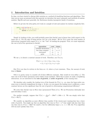
Example 1: For Loop Analysis
Suppose we have the following code sample:
10

11. 1 public void foo(int n) {
2 for (int i = 0; i < n; i++) {
3 for (int j = 0; j < i; j++) {
4 System.out.println(i); //Θ(1) work
5 }
6 }
7 }
Compute T(n) for foo(n) and determine its Big-Θ bound. Constants may be treated as c = Θ(1) terms.
Solution.
T(n) =
n−1
i=0
c +
i−1
j=0
c
= Θ(n) +
n−1
i=0
i−1
j=0
c
= Θ(n) + c
n−1
i=0
i
= Θ(n) + c
1
2
n(n − 1)
= Θ(n) + c n2
− n
= Θ(n) + Θ(n2
) = Θ(n2
)
How else could we analyze this? We know from the loop conditions that we have 0 ≤ j < i < n. Suppose
that we have n boxes in a row. We pick any two boxes, indexed by a and b, where a < b. Let j be the
number of boxes to the left of a, and let i be the number of boxes to the left of b. How many possible ways
can we pick a and b?
n
2
=
1
2
n(n − 1) = Θ(n2
)
We can use a combinatorics approach to some of these problems, as well!
It is important to note that if you can compute an exact T(n), you can prove an immediate Big-Θ. There
may be cases where you can not compute T(n) exactly, which we will see later.
Example 2: For Loop Analysis
Suppose we have another code sample:
1 //Assume n = 2k, k ∈ Z.
2 public void magic(int n) {
3 for (int i = 1; i < n; i *= 2) {
4 System.out.println(i); //Θ(1) work
5 }
6 }
Compute T(n) and determine its Big-Θ bound.
11

12. Solution. We first observe that the outer loop runs a total of log n times.
T(n) = c log n = Θ(log n)
Example 3: A Logarithm and a Factorial Walk Into a Bar...
1 public void mystery(int n) {
2 int count = 0;
3 for (int i = 0; i < n; i++) {
4 for (int j = n; j > 0; j /= 2) {
5 count++;
6 }
7 }
8 }
9
10 //Assume factorial(n) runs in O(1) time.
11 public void mystery2(int n) {
12 int count = 0;
13 for (int i = 0; i < log(factorial(n)); i++) {
14 count++;
15 }
16 }
What are the runtime complexities of mystery(n) and mystery2(n)? Which runs faster than the other?
Prove Big-Oh or Big-Ω, or both.
Solution.
mystery(n) runs in Θ(n log n) time, and mystery2(n) runs in Θ(log n!) time.
Now, let’s examine the functions f(n) = log n! and g(n) = n log n. We will show that log n! ∈ Θ(n log n).
We first show log(n!) is O(n log n). Picking c = 1 and n0 = 1, we have
log(n!) =
n
i=1
log i ≤ n log n
This is clearly true for all n > n0. Therefore, we are done.
We then show that log(n!) is Ω(n log n). Our strategy is to find an easier to work with lower-bound for
log n! that is larger than some cn log n. Then, we can use the transitive property of Big-Ω to achieve our
goal.
log n! = log 1 + log 2 + · · · + log n
≥ log
n
2
+ log(
n
2
+ 1) + · · · + log n delete the first half of the terms
≥
n
2
· log
n
2
replace remaining terms by smallest one
Choosing c = 1
4 and n0 = 4, it is clear that n
2 log n
2 ≥ n
4 log n with some algebraic manipulation:
n
2
log
n
2
≥
n
4
log n
n
2
log n −
n
2
≥
n
4
log n
n log n ≥ 2n
log n ≥ 2
12

13. Therefore, log(n!) is Ω(n log n).
Alternate solution.
We can use Stirling’s formula to prove Big-Θ. For sufficiently large n we can approximate n! as (n
e )n
√
2πn.
log (
n
e
)n
√
2πn = n log n − n + (
1
2
) log(2πn)
, which is Θ(n lg n). We can eyeball this by observing that n log n is the fastest growing term in this sum
(which only contains constant terms, a linear term, and a logarithmic term). We omit a detailed proof.
13