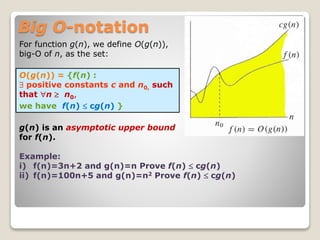
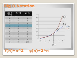
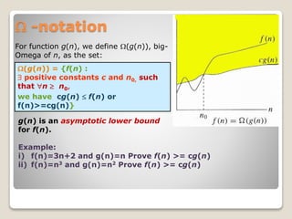
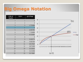
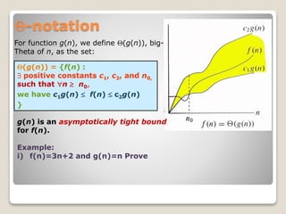
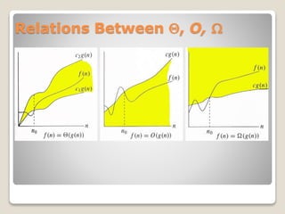
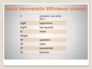
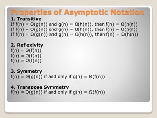
Asymptotic Notations
Introduction
 In mathematics, computer science, and related fields, big O
notation describes the limiting behavior of a function when the
argument tends towards a particular value or infinity, usually in
terms of simpler functions.
 The time complexity of an algorithm quantifies the amount of
time taken by an algorithm to run as a function of the size of the
input to the problem. When it is expressed using big O notation,
the time complexity is said to be described asymptotically, i.e.,
as the input size goes to infinity.
Asymptotic Complexity
 Running time of an algorithm as a function of input size n for large
n.
 Expressed using only the highest-order term in the expression for
the exact running time.
◦ Instead of exact running time, say Q(n2).
 Describes behavior of function in the limit.
 Written using Asymptotic Notation.
 The notations describe different rate-of-growth relations between
the defining function and the defined set of functions.
Big O-notation
O(g(n)) = {f(n) :
 positive constants c and n0, such
that n  n0,
we have f(n)  cg(n) }
For function g(n), we define O(g(n)),
big-O of n, as the set:
g(n) is an asymptotic upper bound
for f(n).
Example:
i) f(n)=3n+2 and g(n)=n Prove f(n)  cg(n)
ii) f(n)=100n+5 and g(n)=n2 Prove f(n)  cg(n)
f(n)=n^2 g(n)=2^n
Big O Notation
 -notation
g(n) is an asymptotic lower bound
for f(n).
Example:
i) f(n)=3n+2 and g(n)=n Prove f(n) >= cg(n)
ii) f(n)=n3 and g(n)=n2 Prove f(n) >= cg(n)
(g(n)) = {f(n) :
 positive constants c and n0, such
that n  n0,
we have cg(n)  f(n) or
f(n)>=cg(n)}
For function g(n), we define (g(n)), big-
Omega of n, as the set:
Big Omega Notation
Q-notation
Q(g(n)) = {f(n) :
 positive constants c1, c2, and n0,
such that n  n0,
we have c1g(n)  f(n)  c2g(n)
}
For function g(n), we define Q(g(n)), big-
Theta of n, as the set:
g(n) is an asymptotically tight bound
for f(n).
Example:
i) f(n)=3n+2 and g(n)=n Prove
Relations Between Q, O, 
Basic Asymptotic Efficiency classes
C constant, we write
O(1)
logN logarithmic
log2N log-squared
N linear
NlogN
N2 quadratic
N3 cubic
2N exponential
N! factorial
Properties of Asymptotic Notation
1. Transitive
If f(n) = Θ(g(n)) and g(n) = Θ(h(n)), then f(n) = Θ(h(n))
If f(n) = O(g(n)) and g(n) = O(h(n)), then f(n) = O(h(n))
If f(n) = Ω(g(n)) and g(n) = Ω(h(n)), then f(n) = Ω(h(n))
2. Reflexivity
f(n) = Θ(f(n))
f(n) = O(f(n))
f(n) = Ω(f(n))
3. Symmetry
f(n) = Θ(g(n)) if and only if g(n) = Θ(f(n))
4. Transpose Symmetry
f(n) = O(g(n)) if and only if g(n) = Ω(f(n))
The End

Asymptotic notation

  • 1.
  • 2.
    Introduction  In mathematics,computer science, and related fields, big O notation describes the limiting behavior of a function when the argument tends towards a particular value or infinity, usually in terms of simpler functions.  The time complexity of an algorithm quantifies the amount of time taken by an algorithm to run as a function of the size of the input to the problem. When it is expressed using big O notation, the time complexity is said to be described asymptotically, i.e., as the input size goes to infinity.
  • 3.
    Asymptotic Complexity  Runningtime of an algorithm as a function of input size n for large n.  Expressed using only the highest-order term in the expression for the exact running time. ◦ Instead of exact running time, say Q(n2).  Describes behavior of function in the limit.  Written using Asymptotic Notation.  The notations describe different rate-of-growth relations between the defining function and the defined set of functions.
  • 4.
    Big O-notation O(g(n)) ={f(n) :  positive constants c and n0, such that n  n0, we have f(n)  cg(n) } For function g(n), we define O(g(n)), big-O of n, as the set: g(n) is an asymptotic upper bound for f(n). Example: i) f(n)=3n+2 and g(n)=n Prove f(n)  cg(n) ii) f(n)=100n+5 and g(n)=n2 Prove f(n)  cg(n)
  • 5.
  • 6.
     -notation g(n) isan asymptotic lower bound for f(n). Example: i) f(n)=3n+2 and g(n)=n Prove f(n) >= cg(n) ii) f(n)=n3 and g(n)=n2 Prove f(n) >= cg(n) (g(n)) = {f(n) :  positive constants c and n0, such that n  n0, we have cg(n)  f(n) or f(n)>=cg(n)} For function g(n), we define (g(n)), big- Omega of n, as the set:
  • 7.
  • 8.
    Q-notation Q(g(n)) = {f(n):  positive constants c1, c2, and n0, such that n  n0, we have c1g(n)  f(n)  c2g(n) } For function g(n), we define Q(g(n)), big- Theta of n, as the set: g(n) is an asymptotically tight bound for f(n). Example: i) f(n)=3n+2 and g(n)=n Prove
  • 9.
  • 10.
    Basic Asymptotic Efficiencyclasses C constant, we write O(1) logN logarithmic log2N log-squared N linear NlogN N2 quadratic N3 cubic 2N exponential N! factorial
  • 11.
    Properties of AsymptoticNotation 1. Transitive If f(n) = Θ(g(n)) and g(n) = Θ(h(n)), then f(n) = Θ(h(n)) If f(n) = O(g(n)) and g(n) = O(h(n)), then f(n) = O(h(n)) If f(n) = Ω(g(n)) and g(n) = Ω(h(n)), then f(n) = Ω(h(n)) 2. Reflexivity f(n) = Θ(f(n)) f(n) = O(f(n)) f(n) = Ω(f(n)) 3. Symmetry f(n) = Θ(g(n)) if and only if g(n) = Θ(f(n)) 4. Transpose Symmetry f(n) = O(g(n)) if and only if g(n) = Ω(f(n))
  • 12.