Download as PDF, PPTX

![3
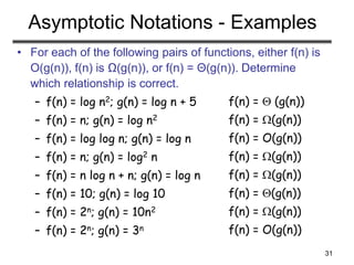
Algorithm Analysis: Example
• Alg.: MIN (a[1], …, a[n])
m ← a[1];
for i ← 2 to n
if a[i] < m
then m ← a[i];
• Running time:
– the number of primitive operations (steps) executed
before termination
T(n) =1 [first step] + (n) [for loop] + (n-1) [if condition] +
(n-1) [the assignment in then] = 3n - 1
• Order (rate) of growth:
– The leading term of the formula
– Expresses the asymptotic behavior of the algorithm](https://image.slidesharecdn.com/asymptotic-180406164005/85/Asymptotic-Notation-3-320.jpg)


![35
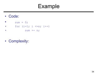
Example
• Code:
• sum = 0;
• for (j=1; j<=n; j++)
• for (i=1; i<=j; i++)
• sum++;
• for (k=0; k<n; k++)
• A[k] = k;
• Complexity:](https://image.slidesharecdn.com/asymptotic-180406164005/85/Asymptotic-Notation-35-320.jpg)


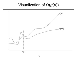
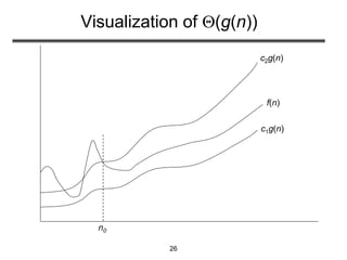
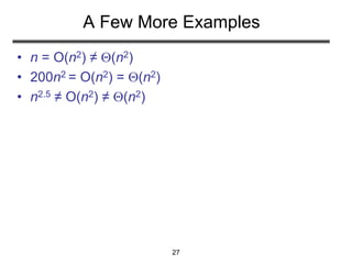
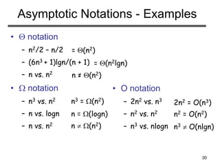
This document discusses analyzing algorithms and asymptotic notation. It defines running time as the number of primitive operations before termination. Examples are provided to illustrate calculating running time functions and classifying them by order of growth such as constant, logarithmic, linear, quadratic, and exponential time. Asymptotic notation such as Big-O, Big-Omega, and Big-Theta are introduced to classify functions by their asymptotic growth rates. Examples are given to demonstrate determining tight asymptotic bounds between functions. Recurrences are defined as equations describing functions in terms of smaller inputs and base cases, which are useful for analyzing recurrent algorithms.