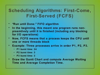
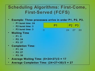
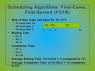
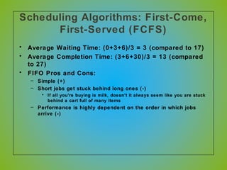
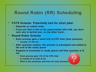
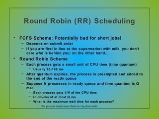
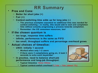
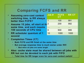
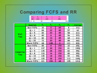
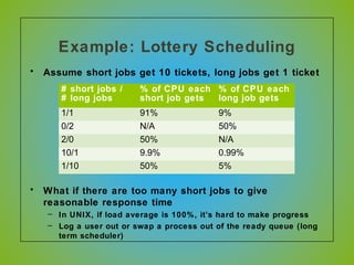
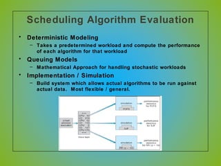
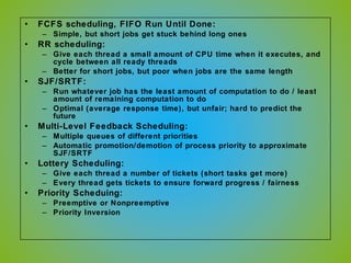
The document discusses various CPU scheduling algorithms used in operating systems including first-come, first-served (FCFS), round robin (RR), shortest job first (SJF), and shortest remaining time first (SRTF). It explains the assumptions, goals, and tradeoffs of each algorithm such as minimizing response time, maximizing throughput, and ensuring fairness. Examples are provided to illustrate how each algorithm works and its performance compared to others under different conditions involving job lengths. Predicting future job lengths is also discussed as it can impact the performance of algorithms like SRTF.
Maximum CPU utilization obtained with multiprogramming
CPU–I/O Burst Cycle – Process execution consists of a cycle of CPU execution and I/O wait
CPU burst followed by I/O burst
CPU burst distribution is of main concern
Hello....
Dear views
Scheduling is most important Role in OS..... in this ppt i described very Creatively about Process Scheduling...... I hope you like it..... and easily understand it...... :-) :-)
It consists of CPU scheduling algorithms, examples, scheduling problems, realtime scheduling algorithms and issues. Multiprocessing and multicore scheduling.
A presentation on different CPU scheduling algorithms such as SJF, RR and FIFO detailed explanation with advantages and disadvantages of each algorithm. This ppt also contains brief information about the multiprocessor scheduling and the performance evaluation of Scheduling algorithms.
Deadlock happens when two threads are waiting for a mutex owned by the other (circular deadlock between multiple threads is also possible). Therefore, we need to check for deadlock only when a thread fails to lock a mutex. At that point, the Thread Manager needs to suspend all threads and take over to perform a cycle check on mutex dependency. Finding such a cycle is easily done by performing a tree traversal of the dependencies, and marking threads and mutexes along the way. Using this method, we can detect deadlock and identify all threads and mutexes involved in the deadlock.
CPU scheduling is the basis of multiprogrammed operating systems. By switching the CPU among processes, the operating system can make the computer more productive
- To introduce CPU scheduling, which is the basis for multiprogrammed operating systems
- To describe various CPU-scheduling algorithms
- To discuss evaluation criteria for selecting a CPU-scheduling algorithm for a particular system
- To examine the scheduling algorithms of several operating systems
POWER GENERATION OF THERMAL POWER PLANTsathish sak
. The kinetic energy of the molecules in a solid, liquid or gas
2. The more kinetic energy, the more thermal energy the object possesses
3. Physicists also call this the internal energy of an object
mathematics application fiels of engineeringsathish sak
MATHS IS HARD
MATHS IS BORING
MATHS HAS NOTHING TO DO WITH REAL LIFE
ALL MATHEMATICIANS ARE MAD!
BUT I CAN SHOW YOU THAT MATHS IS IMPORTANT IN
CRIME DETECTION MEDICINE FINDING LANDMINES
Plastic is a material consists of wide range of synthetic or organics that can be moulded into solid object with diverse shapes.
The word PLASTIC is derived from the Greek Word “PLASTIKOS” meaning capable of being shaped or moulded.
Plastics are organic polymers of higher molecular mass.
Radio frequency identification(RFID) technology using at various application by using radio frequency ranges.
It is especially used at tollgates. For automation of gate control.
It can also used at library systems.
Green Chemistry is the utilisation of a set of principles that reduces or eliminates the use or generation of hazardous substances in the design, manufacture and application of chemical products .
Adjusting primitives for graph : SHORT REPORT / NOTESSubhajit Sahu
Graph algorithms, like PageRank Compressed Sparse Row (CSR) is an adjacency-list based graph representation that is
Multiply with different modes (map)
1. Performance of sequential execution based vs OpenMP based vector multiply.
2. Comparing various launch configs for CUDA based vector multiply.
Sum with different storage types (reduce)
1. Performance of vector element sum using float vs bfloat16 as the storage type.
Sum with different modes (reduce)
1. Performance of sequential execution based vs OpenMP based vector element sum.
2. Performance of memcpy vs in-place based CUDA based vector element sum.
3. Comparing various launch configs for CUDA based vector element sum (memcpy).
4. Comparing various launch configs for CUDA based vector element sum (in-place).
Sum with in-place strategies of CUDA mode (reduce)
1. Comparing various launch configs for CUDA based vector element sum (in-place).
Enhanced Enterprise Intelligence with your personal AI Data Copilot.pdfGetInData
Recently we have observed the rise of open-source Large Language Models (LLMs) that are community-driven or developed by the AI market leaders, such as Meta (Llama3), Databricks (DBRX) and Snowflake (Arctic). On the other hand, there is a growth in interest in specialized, carefully fine-tuned yet relatively small models that can efficiently assist programmers in day-to-day tasks. Finally, Retrieval-Augmented Generation (RAG) architectures have gained a lot of traction as the preferred approach for LLMs context and prompt augmentation for building conversational SQL data copilots, code copilots and chatbots.
In this presentation, we will show how we built upon these three concepts a robust Data Copilot that can help to democratize access to company data assets and boost performance of everyone working with data platforms.
Why do we need yet another (open-source ) Copilot?
How can we build one?
Architecture and evaluation
Techniques to optimize the pagerank algorithm usually fall in two categories. One is to try reducing the work per iteration, and the other is to try reducing the number of iterations. These goals are often at odds with one another. Skipping computation on vertices which have already converged has the potential to save iteration time. Skipping in-identical vertices, with the same in-links, helps reduce duplicate computations and thus could help reduce iteration time. Road networks often have chains which can be short-circuited before pagerank computation to improve performance. Final ranks of chain nodes can be easily calculated. This could reduce both the iteration time, and the number of iterations. If a graph has no dangling nodes, pagerank of each strongly connected component can be computed in topological order. This could help reduce the iteration time, no. of iterations, and also enable multi-iteration concurrency in pagerank computation. The combination of all of the above methods is the STICD algorithm. [sticd] For dynamic graphs, unchanged components whose ranks are unaffected can be skipped altogether.
06-04-2024 - NYC Tech Week - Discussion on Vector Databases, Unstructured Data and AI
Round table discussion of vector databases, unstructured data, ai, big data, real-time, robots and Milvus.
A lively discussion with NJ Gen AI Meetup Lead, Prasad and Procure.FYI's Co-Found
The Building Blocks of QuestDB, a Time Series Databasejavier ramirez
Talk Delivered at Valencia Codes Meetup 2024-06.
Traditionally, databases have treated timestamps just as another data type. However, when performing real-time analytics, timestamps should be first class citizens and we need rich time semantics to get the most out of our data. We also need to deal with ever growing datasets while keeping performant, which is as fun as it sounds.
It is no wonder time-series databases are now more popular than ever before. Join me in this session to learn about the internal architecture and building blocks of QuestDB, an open source time-series database designed for speed. We will also review a history of some of the changes we have gone over the past two years to deal with late and unordered data, non-blocking writes, read-replicas, or faster batch ingestion.
Adjusting OpenMP PageRank : SHORT REPORT / NOTESSubhajit Sahu
For massive graphs that fit in RAM, but not in GPU memory, it is possible to take
advantage of a shared memory system with multiple CPUs, each with multiple cores, to
accelerate pagerank computation. If the NUMA architecture of the system is properly taken
into account with good vertex partitioning, the speedup can be significant. To take steps in
this direction, experiments are conducted to implement pagerank in OpenMP using two
different approaches, uniform and hybrid. The uniform approach runs all primitives required
for pagerank in OpenMP mode (with multiple threads). On the other hand, the hybrid
approach runs certain primitives in sequential mode (i.e., sumAt, multiply).
Levelwise PageRank with Loop-Based Dead End Handling Strategy : SHORT REPORT ...Subhajit Sahu
Abstract — Levelwise PageRank is an alternative method of PageRank computation which decomposes the input graph into a directed acyclic block-graph of strongly connected components, and processes them in topological order, one level at a time. This enables calculation for ranks in a distributed fashion without per-iteration communication, unlike the standard method where all vertices are processed in each iteration. It however comes with a precondition of the absence of dead ends in the input graph. Here, the native non-distributed performance of Levelwise PageRank was compared against Monolithic PageRank on a CPU as well as a GPU. To ensure a fair comparison, Monolithic PageRank was also performed on a graph where vertices were split by components. Results indicate that Levelwise PageRank is about as fast as Monolithic PageRank on the CPU, but quite a bit slower on the GPU. Slowdown on the GPU is likely caused by a large submission of small workloads, and expected to be non-issue when the computation is performed on massive graphs.
Analysis insight about a Flyball dog competition team's performanceroli9797
Insight of my analysis about a Flyball dog competition team's last year performance. Find more: https://github.com/rolandnagy-ds/flyball_race_analysis/tree/main
2. CPU Scheduling
• How is the OS to decide which of several tasks to take
off a queue?
• Scheduling: deciding which threads are given access to
resources from moment to moment.
3. Assumptions about Scheduling
• CPU scheduling big area of research in early ‘70s
• Many implicit assumptions for CPU scheduling:
– One program per user
– One thread per program
– Programs are independent
• These are unrealistic but simplify the problem
• Does “fair” mean fairness among users or programs?
– If I run one compilation job and you run five, do you get five
times as much CPU?
• Often times, yes!
• Goal: dole out CPU time to optimize some desired
parameters of the system.
– What parameters?
5. Assumption: CPU Bursts
• Execution model: programs alternate between bursts of
CPU and I/O
– Program typically uses the CPU for some period of time, then
does I/O, then uses CPU again
– Each scheduling decision is about which job to give to the CPU
for use by its next CPU burst
– With timeslicing, thread may be forced to give up CPU before
finishing current CPU burst.
6. What is Important in a Scheduling
Algorithm?
• Minimize Response Time
– Elapsed time to do an operation (job)
– Response time is what the user sees
• Time to echo keystroke in editor
• Time to compile a program
• Real-time Tasks: Must meet deadlines imposed by World
• Maximize Throughput
– Jobs per second
– Throughput related to response time, but not identical
• Minimizing response time will lead to more context switching than if
you maximized only throughput
– Minimize overhead (context switch time) as well as efficient
use of resources (CPU, disk, memory, etc.)
• Fairness
– Share CPU among users in some equitable way
– Not just minimizing average response time
7. Scheduling Algorithms: First-Come,
First-Served (FCFS)
• “Run until Done:” FIFO algorithm
• In the beginning, this meant one program runs non-
preemtively until it is finished (including any blocking
for I/O operations)
• Now, FCFS means that a process keeps the CPU until
one or more threads block
• Example: Three processes arrive in order P1, P2, P3.
– P1 burst time: 24
– P2 burst time: 3
– P3 burst time: 3
• Draw the Gantt Chart and compute Average Waiting
Time and Average Completion Time.
10. Scheduling Algorithms: First-Come,
First-Served (FCFS)
• What if their order had been P2, P3, P1?
– P1 burst time: 24
– P2 burst time: 3
– P3 burst time: 3
• Waiting Time
– P1: 0
– P2: 3
– P3: 6
• Completion Time:
– P1: 3
– P2: 6
– P3: 30
• Average Waiting Time: (0+3+6)/3 = 3 (compared to 17)
• Average Completion Time: (3+6+30)/3 = 13 (compared
to 27)
P1P2 P3
0 3 6 30
11. Scheduling Algorithms: First-Come,
First-Served (FCFS)
• Average Waiting Time: (0+3+6)/3 = 3 (compared to 17)
• Average Completion Time: (3+6+30)/3 = 13 (compared
to 27)
• FIFO Pros and Cons:
– Simple (+)
– Short jobs get stuck behind long ones (-)
• If all you’re buying is milk, doesn’t it always seem like you are stuck
behind a cart full of many items
– Performance is highly dependent on the order in which jobs
arrive (-)
12. Round Robin (RR) Scheduling
• FCFS Scheme: Potentially bad for short jobs!
– Depends on submit order
– If you are first in line at the supermarket with milk, you don’t
care who is behind you; on the other hand…
• Round Robin Scheme
– Each process gets a small unit of CPU time (time quantum)
• Usually 10-100 ms
– After quantum expires, the process is preempted and added to
the end of the ready queue
– Suppose N processes in ready queue and time quantum is Q
ms:
• Each process gets 1/N of the CPU time
• In chunks of at most Q ms
• What is the maximum wait time for each process?
13. Round Robin (RR) Scheduling
• FCFS Scheme: Potentially bad for short jobs!
– Depends on submit order
– If you are first in line at the supermarket with milk, you don’t
care who is behind you; on the other hand…
• Round Robin Scheme
– Each process gets a small unit of CPU time (time quantum)
• Usually 10-100 ms
– After quantum expires, the process is preempted and added to
the end of the ready queue
– Suppose N processes in ready queue and time quantum is Q
ms:
• Each process gets 1/N of the CPU time
• In chunks of at most Q ms
• What is the maximum wait time for each process?
– No process waits more than (n-1)q time units
14. Round Robin (RR) Scheduling
• Round Robin Scheme
– Each process gets a small unit of CPU time (time quantum)
• Usually 10-100 ms
– After quantum expires, the process is preempted and added to
the end of the ready queue
– Suppose N processes in ready queue and time quantum is Q
ms:
• Each process gets 1/N of the CPU time
• In chunks of at most Q ms
• What is the maximum wait time for each process?
– No process waits more than (n-1)q time units
• Performance Depends on Size of Q
– Small Q => interleaved
– Large Q is like…
– Q must be large with respect to context switch time, otherwise
overhead is too high (spending most of your time context
switching!)
15. Round Robin (RR) Scheduling
• Round Robin Scheme
– Each process gets a small unit of CPU time (time quantum)
• Usually 10-100 ms
– After quantum expires, the process is preempted and added to
the end of the ready queue
– Suppose N processes in ready queue and time quantum is Q
ms:
• Each process gets 1/N of the CPU time
• In chunks of at most Q ms
• What is the maximum wait time for each process?
– No process waits more than (n-1)q time units
• Performance Depends on Size of Q
– Small Q => interleaved
– Large Q is like FCFS
– Q must be large with respect to context switch time, otherwise
overhead is too high (spending most of your time context
switching!)
16. Example of RR with Time Quantum
= 4
Process Burst Time
P1 24
P2 3
P3 3
• The Gantt chart is:
P1 P2 P3 P1 P1 P1 P1 P1
0 4 7 10 14 1822 26 30
17. Example of RR with Time Quantum
= 4
Process Burst Time
P1 24
P2 3
P3 3
• Waiting Time:
– P1: (10-4) = 6
– P2: (4-0) = 4
– P3: (7-0) = 7
• Completion Time:
– P1: 30
– P2: 7
– P3: 10
• Average Waiting Time: (6 + 4 + 7)/3= 5.67
• Average Completion Time: (30+7+10)/3=15.67
P1 P2 P3 P1 P1 P1 P1 P1
0 4 7 10 14 1822 26 30
19. Example of RR with Time Quantum
= 20
• Waiting Time:
– P1: (68-20)+(112-88) = 72
– P2: (20-0) = 20
– P3: (28-0)+(88-48)+(125-108) = 85
– P4: (48-0)+(108-68) = 88
• Completion Time:
– P1: 125
– P2: 28
– P3: 153
– P4: 112
• Average Waiting Time: (72+20+85+88)/4 = 66.25
• Average Completion Time: (125+28+153+112)/4 =
104.5
A process can finish before the time quantum expires, and release the CPU.
20. RR Summary
• Pros and Cons:
– Better for short jobs (+)
– Fair (+)
– Context-switching time adds up for long jobs (-)
• The previous examples assumed no additional time was needed for
context switching – in reality, this would add to wait and completion
time without actually progressing a process towards completion.
• Remember: the OS consumes resources, too!
• If the chosen quantum is
– too large, response time suffers
– infinite, performance is the same as FIFO
– too small, throughput suffers and percentage overhead grows
• Actual choices of timeslice:
– UNIX: initially 1 second:
• Worked when only 1-2 users
• If there were 3 compilations going on, it took 3
seconds to echo each keystroke!
– In practice, need to balance short-job
performance and long-job throughput:
• Typical timeslice 10ms-100ms
• Typical context-switch overhead 0.1ms – 1ms (about 1%)
21. Comparing FCFS and RR
• Assuming zero-cost context
switching time, is RR always
better than FCFS?
• Assume 10 jobs, all start at the
same time, and each require
100 seconds of CPU time
• RR scheduler quantum of 1
second
• Completion Times (CT)
– Both FCFS and RR finish at the same time
– But average response time is much worse under RR!
• Bad when all jobs are same length
• Also: cache state must be shared between all jobs with
RR but can be devoted to each job with FIFO
– Total time for RR longer even for zero-cost context switch!
Job # FCFS
CT
RR CT
1 100 991
2 200 992
… … …
9 900 999
10 1000 1000
23. Scheduling
• The performance we get is somewhat dependent on
what “kind” of jobs we are running (short jobs, long
jobs, etc.)
• If we could “see the future,” we could mirror best FCFS
• Shortest Job First (SJF) a.k.a. Shortest Time to
Completion First (STCF):
– Run whatever job has the least amount of computation to do
• Shortest Remaining Time First (SRTF) a.k.a. Shortest
Remaining Time to Completion First (SRTCF):
– Preemptive version of SJF: if a job arrives and has a shorter
time to completion than the remaining time on the current job,
immediately preempt CPU
• These can be applied either to a whole program or the
current CPU burst of each program
– Idea: get short jobs out of the system
– Big effect on short jobs, only small effect on long ones
– Result: better average response time
24. Scheduling
• But, this is hard to estimate
• We could get feedback from the program or the user,
but they have incentive to lie!
• SJF/SRTF are the best you can do at minimizing
average response time
– Provably optimal (SJF among non-preemptive, SRTF among
preemptive)
– Since SRTF is always at least as good as SJF, focus on SRTF
• Comparison of SRTF with FCFS and RR
– What if all jobs are the same length?
– What if all jobs have varying length?
25. Scheduling
• But, this is hard to estimate
• We could get feedback from the program or the user,
but they have incentive to lie!
• SJF/SRTF are the best you can do at minimizing
average response time
– Provably optimal (SJF among non-preemptive, SRTF among
preemptive)
– Since SRTF is always at least as good as SJF, focus on SRTF
• Comparison of SRTF with FCFS and RR
– What if all jobs are the same length?
• SRTF becomes the same as FCFS (i.e. FCFS is the best we can do)
– What if all jobs have varying length?
• SRTF (and RR): short jobs are not stuck behind long ones
26. Example: SRTF
• A,B: both CPU bound, run for a week
• C: I/O bound, loop 1ms CPU, 9ms disk I/O
• If only one at a time, C uses 90% of the disk, A or B
could use 100% of the CPU
• With FIFO: Once A and B get in, the CPU is held for
two weeks
• What about RR or SRTF?
– Easier to see with a timeline
A or B C C I/O
27. Example: SRTF
• A,B: both CPU bound, run for a week
• C: I/O bound, loop 1ms CPU, 9ms disk I/O
A or B C C I/O
28. Last Word on SRTF
• Starvation
– SRTF can lead to starvation if many small jobs!
– Large jobs never get to run
• Somehow need to predict future
– How can we do this?
– Some systems ask the user
• When you submit a job, you have to say how long it will take
• To stop cheating, system kills job if it takes too long
– But even non-malicious users have trouble predicting runtime
of their jobs
• Bottom line, can’t really tell how long job will take
– However, can use SRTF as a yardstick for measuring other
policies, since it is optimal
• SRTF Pros and Cons
– Optimal (average response time) (+)
– Hard to predict future (-)
– Unfair, even though we minimized average response time! (-)
29. Predicting the Future
• Back to predicting the future… perhaps we can predict
the next CPU burst length?
• Iff programs are generally repetitive, then they may be
predictable
• Create an adaptive policy that changes based on past
behavior
– CPU scheduling, virtual memory, file systems, etc.
– If program was I/O bound in the past, likely in the future
• Example: SRTF with estimated burst length
– Use an estimator function on previous bursts
– Let T(n-1), T(n-2), T(n-3), …, be previous burst lengths.
Estimate next burst T(n) = f(T(n-1), T(n-2), T(n-3),…)
– Function f can be one of many different time series estimation
schemes (Kalman filters, etc.)
30. Determining Length of Next CPU
Burst
• Can only estimate the length
• Can be done by using the length of previous CPU
bursts, using exponential averaging
:Define4.
10,3.
burstCPUnexttheforvaluepredicted2.
burstCPUoflengthactual1.
≤≤
=
=
+
αα
τ 1n
th
n nt
( ) .11 nnn t ταατ −+=+
32. Examples of Exponential
Averaging
∀ α =0
τn+1 = τn
– Recent history does not count
∀ α =1
– τn+1 = α tn
– Only the actual last CPU burst counts
• If we expand the formula, we get:
τn+1 = α tn+(1 - α)α tn -1 + …
+(1 - α )j
α tn -j + …
+(1 - α )n +1
τ0
• Since both α and (1 - α) are less than or equal to 1,
each successive term has less weight than its
predecessor
33. Priority Scheduling
• A priority number (integer) is associated with each
process
• The CPU is allocated to the process with the highest
priority (smallest integer ≡ highest priority)
– Preemptive (if a higher priority process enters, it receives the
CPU immediately)
– Nonpreemptive (higher priority processes must wait until the
current process finishes; then, the highest priority ready
process is selected)
• SJF is a priority scheduling where priority is the
predicted next CPU burst time
• Problem ≡ Starvation – low priority processes may
never execute
• Solution ≡ Aging – as time progresses increase the
priority of the process
34. Priority Inversion
• Consider a scenario in which there are three
processes, one with high priority (H), one with medium
priority (M), and one with low priority (L).
• Process L is running and successfully acquires a
resource, such as a lock or semaphore.
• Process H begins; since we are using a preemptive
priority scheduler, process L is preempted for process
H.
• Process H tries to acquire L’s resource, and blocks
(because it is held by L).
• Process M begins running, and, since it has a higher
priority than L, it is the highest priority ready process.
It preempts L and runs, thus starving high priority
process H.
• This is known as priority inversion.
• What can we do?
35. Priority Inversion
• Process L should, in fact, be temporarily of “higher
priority” than process M, on behalf of process H.
• Process H can donate its priority to process L, which,
in this case, would make it higher priority than process
M.
• This enables process L to preempt process M and run.
• When process L is finished, process H becomes
unblocked.
• Process H, now being the highest priority ready
process, runs, and process M must wait until it is
finished.
• Note that if process M’s priority is actually higher than
process H, priority donation won’t be sufficient to
increase process L’s priority above process M. This is
expected behavior (after all, process M would be “more
important” in this case than process H).
36. Multi-level Feedback Scheduling
• Another method for exploiting past behavior
– Multiple queues, each with different priority
• Higher priority queues often considered “foreground” tasks
– Each queue has its own scheduling algorithm
• E.g. foreground RR, background FCFS
• Sometimes multiple RR priorities with quantum increasing
exponentially (highest queue: 1ms, next: 2ms, next: 4ms, etc.)
– Adjust each job’s priority as follows (details vary)
• Job starts in highest priority queue
• If entire CPU time quantum expires, drop one level
• If CPU is yielded during the quantum, push up one level (or to top)
37. Scheduling Details
• Result approximates SRTF
– CPU bound jobs drop rapidly to lower queues
– Short-running I/O bound jobs stay near the top
• Scheduling must be done between the queues
– Fixed priority scheduling: serve all from the highest priority,
then the next priority, etc.
– Time slice: each queue gets a certain amount of CPU time
(e.g., 70% to the highest, 20% next, 10% lowest)
• Countermeasure: user action that can foil intent of the
OS designer
– For multilevel feedback, put in a bunch of meaningless I/O to
keep job’s priority high
– But if everyone does this, it won’t work!
– Consider an Othello program, playing against a competitor.
Key was to compute at a higher priority than the competitors.
• Put in printf’s, run much faster!
38. Scheduling Details
• It is apparent that scheduling is facilitated by having a
“good mix” of I/O bound and CPU bound programs, so
that there are long and short CPU bursts to prioritize
around.
• There is typically a long-term and a short-term
scheduler in the OS.
• We have been discussing the design of the short-term
scheduler.
• The long-term scheduler decides what processes
should be put into the ready queue in the first place for
the short-term scheduler, so that the short-term
scheduler can make fast decisions on a good mix of a
subset of ready processes.
• The rest are held in memory or disk
– Why else is this helpful?
39. Scheduling Details
• It is apparent that scheduling is facilitated by having a
“good mix” of I/O bound and CPU bound programs, so
that there are long and short CPU bursts to prioritize
around.
• There is typically a long-term and a short-term
scheduler in the OS.
• We have been discussing the design of the short-term
scheduler.
• The long-term scheduler decides what processes
should be put into the ready queue in the first place for
the short-term scheduler, so that the short-term
scheduler can make fast decisions on a good mix of a
subset of ready processes.
• The rest are held in memory or disk
– This also provides more free memory for the subset of ready
processes given to the short-term scheduler.
40. Fairness
• What about fairness?
– Strict fixed-policy scheduling between queues is unfair (run
highest, then next, etc.)
• Long running jobs may never get the CPU
• In Multics, admins shut down the machine and found a 10-year-old
job
– Must give long-running jobs a fraction of the CPU even when
there are shorter jobs to run
• Tradeoff: fairness gained by hurting average response time!
• How to implement fairness?
– Could give each queue some fraction of the CPU
• i.e., for one long-running job and 100 short-running ones?
• Like express lanes in a supermarket – sometimes express lanes get
so long, one gets better service by going into one of the regular
lines
– Could increase priority of jobs that don’t get service (as seen in
the multilevel feedback example)
• This was done in UNIX
• Ad hoc – with what rate should priorities be increased?
• As system gets overloaded, no job gets CPU time, so everyone
increases in priority
– Interactive processes suffer
41. Lottery Scheduling
• Yet another alternative: Lottery Scheduling
– Give each job some number of lottery tickets
– On each time slice, randomly pick a winning ticket
– On average, CPU time is proportional to number of tickets
given to each job over time
• How to assign tickets?
– To approximate SRTF, short-running jobs get more, long
running jobs get fewer
– To avoid starvation, every job gets at least one ticket
(everyone makes progress)
• Advantage over strict priority scheduling: behaves
gracefully as load changes
– Adding or deleting a job affects all jobs proportionally,
independent of how many tickets each job possesses
42. Example: Lottery Scheduling
• Assume short jobs get 10 tickets, long jobs get 1 ticket
• What percentage of time does each long job get? Each
short job?
• What if there are too many short jobs to give
reasonable response time
– In UNIX, if load average is 100%, it’s hard to make progress
– Log a user out or swap a process out of the ready queue (long
term scheduler)
43. Example: Lottery Scheduling
• Assume short jobs get 10 tickets, long jobs get 1 ticket
• What if there are too many short jobs to give
reasonable response time
– In UNIX, if load average is 100%, it’s hard to make progress
– Log a user out or swap a process out of the ready queue (long
term scheduler)
# short jobs /
# long jobs
% of CPU each
short job gets
% of CPU each
long job gets
1/1 91% 9%
0/2 N/A 50%
2/0 50% N/A
10/1 9.9% 0.99%
1/10 50% 5%
44. Scheduling Algorithm Evaluation
• Deterministic Modeling
– Takes a predetermined workload and compute the performance
of each algorithm for that workload
• Queuing Models
– Mathematical Approach for handling stochastic workloads
• Implementation / Simulation
– Build system which allows actual algorithms to be run against
actual data. Most flexible / general.
45. Conclusion
• Scheduling: selecting a waiting process
from the ready queue and allocating the
CPU to it
• When do the details of the scheduling
policy and fairness really matter?
– When there aren’t enough resources to go around
• When should you simply buy a faster computer?
– Or network link, expanded highway, etc.
– One approach: buy it when it will pay for itself in improved
response time
• Assuming you’re paying for worse response in reduced productivity,
customer angst, etc.
• Might think that you should buy a faster X when X is utilized 100%,
but usually, response time goes to infinite as utilization goes to
100%
– Most scheduling algorithms work fine in the “linear” portion of
the load curve, and fail otherwise
– Argues for buying a faster X when utilization is at the “knee” of
the curve
46. • FCFS scheduling, FIFO Run Until Done:
– Simple, but short jobs get stuck behind long ones
• RR scheduling:
– Give each thread a small amount of CPU time when it executes, and
cycle between all ready threads
– Better for short jobs, but poor when jobs are the same length
• SJF/SRTF:
– Run whatever job has the least amount of computation to do / least
amount of remaining computation to do
– Optimal (average response time), but unfair; hard to predict the
future
• Multi-Level Feedback Scheduling:
– Multiple queues of different priorities
– Automatic promotion/demotion of process priority to approximate
SJF/SRTF
• Lottery Scheduling:
– Give each thread a number of tickets (short tasks get more)
– Every thread gets tickets to ensure forward progress / fairness
• Priority Scheduing:
– Preemptive or Nonpreemptive
– Priority Inversion