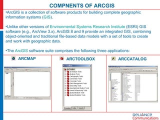
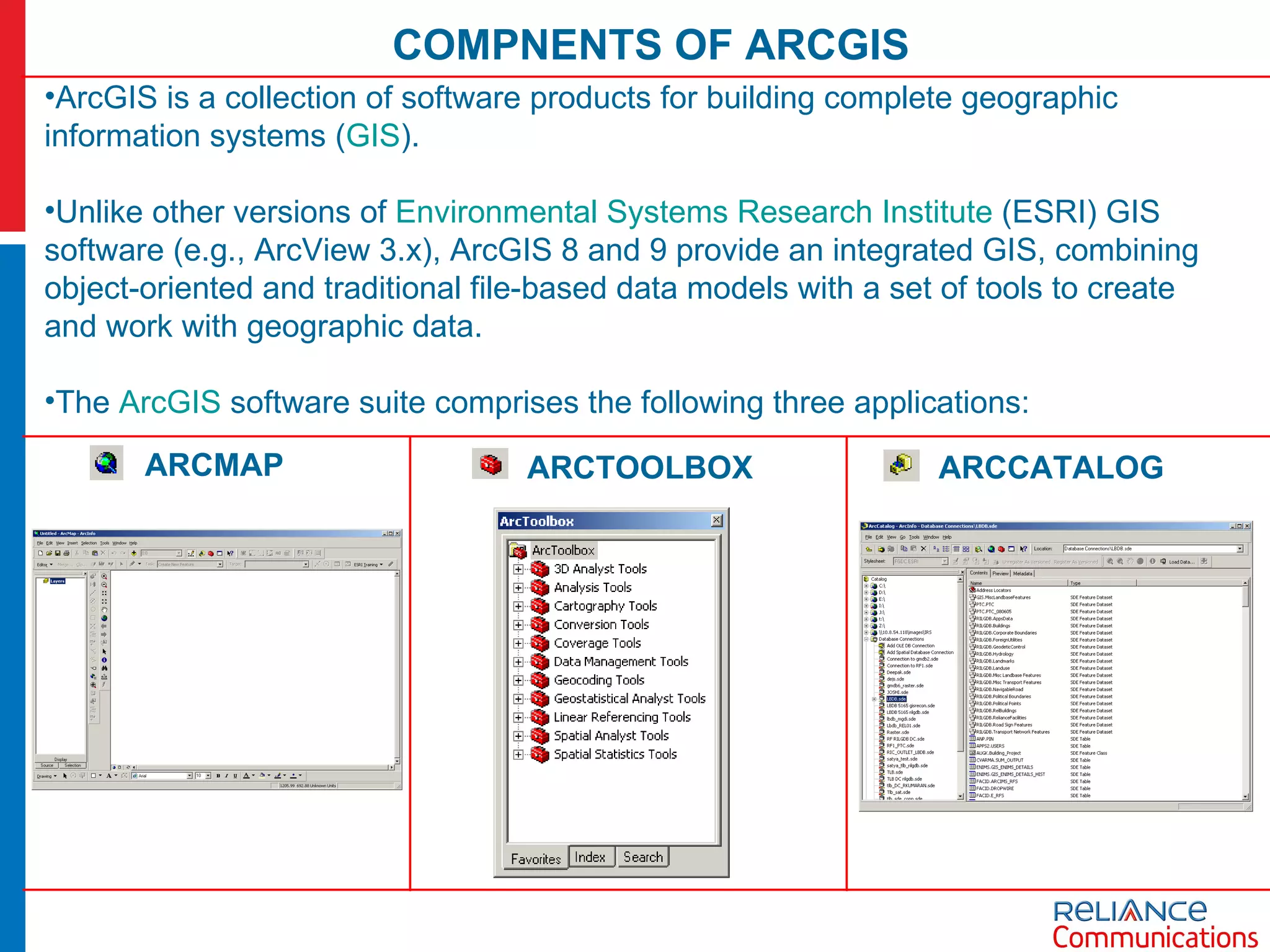
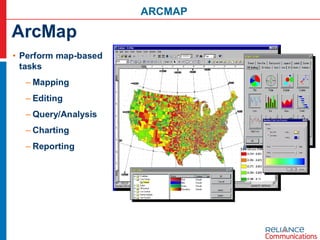
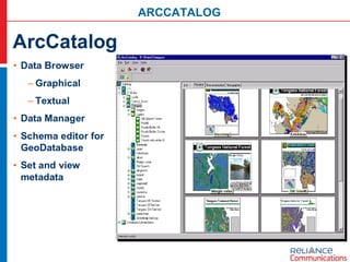
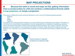
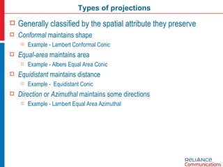
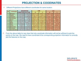
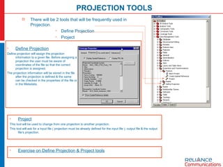
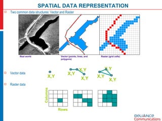
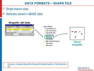
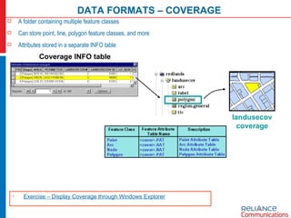
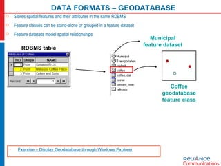
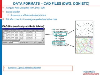
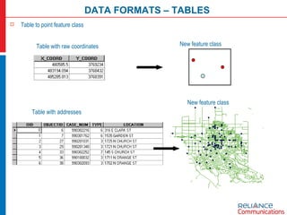
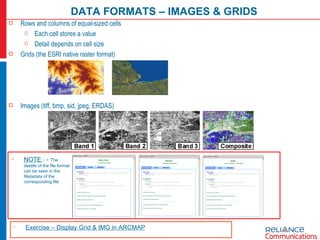
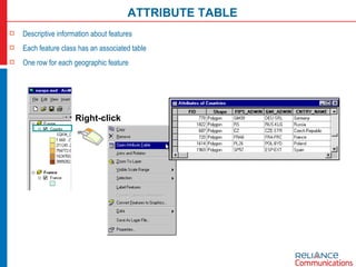
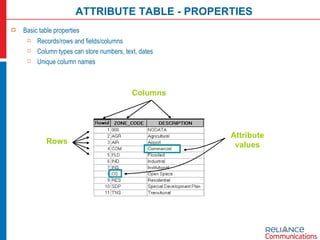
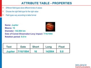
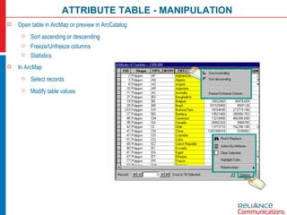
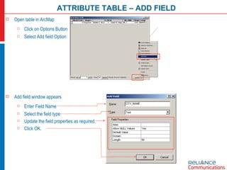
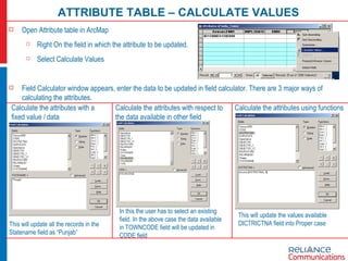
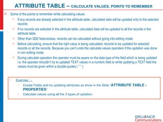
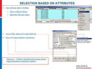
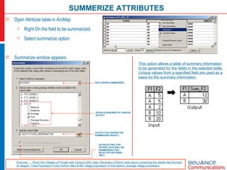
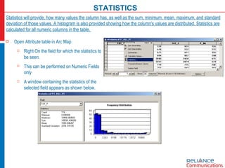
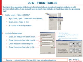
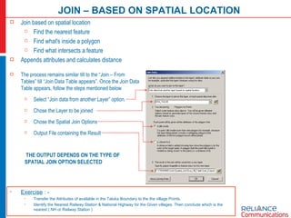
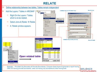
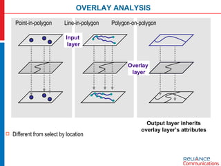
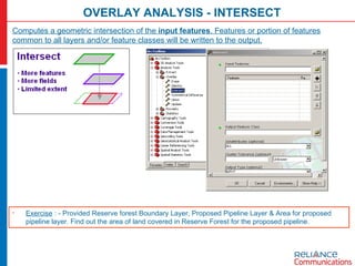
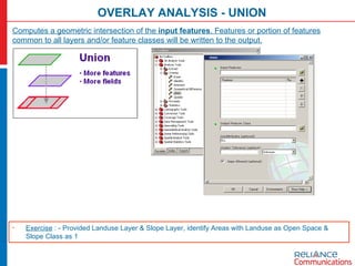
COMPNENTS OF ARCGIS ArcGIS is a collection of software products for building complete geographic information systems ( GIS ). Unlike other versions of  Environmental Systems Research Institute  (ESRI) GIS software (e.g., ArcView 3.x), ArcGIS 8 and 9 provide an integrated GIS, combining object-oriented and traditional file-based data models with a set of tools to create and work with geographic data.  The  ArcGIS  software suite comprises the following three applications: ARCMAP ARCTOOLBOX ARCCATALOG
ARCMAP
ARCTOOLBOX
ARCCATALOG
MAP PROJECTIONS Because the earth is round and maps are flat, getting information from a curved surface to a flat one involves a mathematical formula called a  map projection , or simply a projection.  This process of flattening the earth will cause distortions in one or more of the following spatial properties:  Distance  Area  Shape  Direction  No projection can preserve all these properties; as a result, all flat maps are distorted to some degree. Fortunately, you can choose from many different map projections. Each is distinguished by its suitability for representing a particular portion and amount of the earth's surface and by its ability to preserve distance, area, shape, or direction. Some map projections minimize distortion in one property at the expense of another, while others strive to balance the overall distortion. As a mapmaker, you can decide which properties are most important and choose a projection that suits your needs. South America in selected projections at identical scale.
Types of projections Generally classified by the spatial attribute they preserve Conformal  maintains shape Example - Lambert Conformal Conic Equal-area  maintains area Example - Albers Equal Area Conic Equidistant  maintains distance Example -  Equidistant Conic Direction  or  Azimuthal  maintains some directions Example - Lambert Equal Area Azimuthal
PROJECTION & COODINATES Different Projections have different coordinates for same location. From the above table its very clear that only coordinate information will not be sufficient to plot the points on the map. We need to have coordinate & the corresponding projection information to correctly plot the features on the map.
PROJECTION TOOLS There will be 2 tools that will be frequently used in Projection. Define Projection Project Define Projection Define projection will assign the projection information to a given file. Before assigning a projection the user must be aware of coordinates of the file so that the correct projection is assigned. The projection information will be stored in the file after the projection is defined & the same can be checked in the properties of the file or in the Metadata. Project This tool will be used to change from one projection to another projection. This tool will ask for a input file ( projection must be already defined for the input file ), output file & the output file’s projection. Exercise on Define Projection & Project tools
SPATIAL DATA REPRESENTATION Vector data Raster data Two common data structures: Vector and Raster Real world Vector (points, lines, and polygons) Raster (grid cells) Rows Columns X,Y X,Y X,Y X,Y X,Y X,Y X,Y
SPATIAL DATA FORMATS ArcGIS can work with spatial data in multiple formats CAD Coverage Geodatabase Shapefile Raster Tables ArcGIS
DATA FORMATS – SHAPE FILE Single feature class Attributes stored in dBASE table Donut shapefile Exercise – Display Shape file through Windows Explorer. File Renaming etc Shapefile .dbf table
DATA FORMATS – COVERAGE A folder containing multiple feature classes Can store point, line, polygon feature classes, and more Attributes stored in a separate INFO table landusecov coverage Coverage INFO table Exercise – Display Coverage through Windows Explorer
DATA FORMATS – GEODATABASE Stores spatial features and their attributes in the same RDBMS Feature classes can be stand-alone or grouped in a feature dataset Feature datasets model spatial relationships RDBMS table Coffee geodatabase feature class Municipal feature dataset Exercise – Display Geodatabase through Windows Explorer
DATA FORMATS – CAD FILES (DWG, DGN ETC) Computer Aided Design files (DXF, DWG, DGN) Logical collection  Access one or all feature class(es) at a time Edit after conversion to coverage or geodatabase feature class CAD file (read-only attribute tables)  Exercise – Open Cad file in ARCMAP
DATA FORMATS – TABLES Table to point feature class Table with raw coordinates Table with addresses New feature class New feature class
DATA FORMATS – IMAGES & GRIDS Rows and columns of equal-sized cells  Each cell stores a value Detail depends on cell size Grids (the ESRI native raster format) Images (tiff, bmp, sid, jpeg, ERDAS) Exercise – Display Grid & IMG in ARCMAP NOTE  : -  The details of the file format can be seen in the Metadata of the corresponding file
ATTRIBUTE TABLE Descriptive information about features Each feature class has an associated table One row for each geographic feature Right-click
ATTRIBUTE TABLE - PROPERTIES Basic table properties Records/rows and fields/columns Column types can store numbers, text, dates Unique column names Columns Rows Attribute values
ATTRIBUTE TABLE - PROPERTIES Different field types store different kinds of values Choose the right field type for the right value Field types vary according to table format Name:  Jupiter Moons:  16 Diameter:  142,984 km Date of Comet Shoemaker-Levy impact:  7/16/1994 Rotation period:  9.8 hr Text Date Short Long Float Jupiter 7/16/1994 16 142984 9.8
ATTRIBUTE TABLE - MANIPULATION Open table in ArcMap or preview in ArcCatalog Sort ascending or descending  Freeze/Unfreeze columns Statistics In ArcMap Select records Modify table values
ATTRIBUTE TABLE – ADD FIELD Open table in ArcMap Click on Options Button  Select Add field Option Add field window appears Enter Field Name  Select the field type Update the field properties as required. Click OK.
ATTRIBUTE TABLE – CALCULATE VALUES Open Attribute table in ArcMap Right On the field in which the attribute to be updated.  Select Calculate Values  Field Calculator window appears, enter the data to be updated in field calculator. There are 3 major ways of calculating the attributes. Calculate the attributes with a fixed value / data This will update all the records in the Statename field as “Punjab” Calculate the attributes with respect to the data available in other field In this the user has to select an existing field. In the above case the data available in TOWNCODE field will be updated in CODE field Calculate the attributes using functions This will update the values available DICTRICTNA field into Proper case
Some of the points to remember while calculating values If any records are already selected in the attribute table, calculated data will be updated only to the selected records  If no records are selected in the attribute table, calculated data will be updated to all the records in the attribute table. Other than SDE featureclass, records can be calculated without going into editing mode. Before calculating, ensure that the right value is being calculated, records to be updated for selected records or all the records. Because you can’t undo the calculate values operation if the updation was done in non editing mode. During calculate operation the operator must be aware on the data type of the field which is being updated i.e. the operator shouldn’t try to updated TEXT values in a numeric field or while updating a TEXT field the values must be given within a double quotes ( “ ” ). ATTRIBUTE TABLE –  CALCULATE VALUES, POINTS TO REMEMBER Exercise : -  Create Fields and try updating attributes as show in the Slide “ ATTRIBUTE TABLE - PROPERTIES “ Calculate values using all the 3 types of updation.
SELECTION BASED ON ATTRIBUTES Open attribute table in ArcMap Click on Options Button  Select By Attributes option Use an SQL statement to select features Save and reload selection expressions SELECTION METHOD Exercise : -  Perform attribute query using various logical operators & selection method
SUMMERIZE ATTRIBUTES Open Attribute table in ArcMap Right On the field to be summarized.  Select summarize option Summarize window appears FIELD BEING SUMMARIZED OUTPUT FILE HAVING THE SUMMERIZED RESULT DETAILS REQUIRED BY USER IN OUTPUT ON SELECTING THIS OPTION, DATA WILL BE SUMMARIZED FOR SELECTED RECORDS ONLY This option allows a table of summary information to be generated for the fields in the selected table. Unique values from a specified field are used as a basis for the summary information.   Exercise : -  Given the Villages of Punjab with Census 2001 data. Generate a District wise report containing the details like Number of villages, Total Population in the District, Max & Min village population in that district, average village population.
STATISTICS Open Attribute table in Arc Map Right On the field for which the statistics to be seen.  This can be performed on Numeric Fields only A window containing the statistics of the selected field appears as shown below. Statistics will provide, how many values the column has, as well as the sum, minimum, mean, maximum, and standard deviation of those values. A histogram is also provided showing how the column's values are distributed. Statistics are calculated for all numeric columns in the table.
JOIN – FROM TABLES Add the Layers / Tables in ARCMAP Right On the Layers / Tables which is to be joined. Select Joins & Relate    Join A Join data table window appears. Joining involves appending fields (items) of one table to those of another through an attributes or field common to both tables. A join is usually used to attach more attributes to the attribute table of a geographic layer Join Data Table appears Select Join attribute from a table option. Chose the common field in the Input file Chose the Layer / Table to be joined Chose the common field in the join file Click on Advanced button Select options like “Keep All Records” or “Keep Only Matching Records” Type of outputs on selecting each option is shown below Exercise : - Join attributes of Census 2001 data with Village locations
JOIN – BASED ON SPATIAL LOCATION Exercise  : - Transfer the Attributes of available in the Taluka Boundary to the the village Points. Identify the Nearest Railway Station & National Highway for the Given villages. Then conclude which is the nearest ( NH or Railway Station ) The process remains similar till to the “Join – From Tables” till “Join Data Table appears”. Once the Join Data Table appears, follow the steps mentioned below Select “Join data from another Layer” option. Chose the Layer to be joined Chose the Spatial Join Options Output File containing the Result THE OUTPUT DEPENDS ON THE TYPE OF SPATIAL JOIN OPTION SELECTED Join based on spatial location Find the nearest feature Find what's inside a polygon Find what intersects a feature Appends attributes and calculates distance
RELATE Define relationship between two tables. Tables remain independent   Add the Layers / Tables in ARCMAP Right On the Layers / Tables which is to be related. Select Joins & Relate    Relate A  Relate window appears. COMMON FIELD IN THE INPUT FILE COMMON FIELD IN RELATE FILE RELATE FILE RELATE NAME Open related table Exercise  : - Provided City Boundary & Pincode Boundaries. Compare these layers & generate a report having cities not having pincode boundaries, cities not having city boundaries & cities having both.
Point-in-polygon  Line-in-polygon  Polygon-on-polygon Different from select by location Output layer inherits overlay layer’s attributes OVERLAY ANALYSIS Overlay  layer Input  layer
OVERLAY ANALYSIS - INTERSECT Computes a geometric intersection of the  input features . Features or portion of features common to all layers and/or feature classes will be written to the output. Exercise  : - Provided Reserve forest Boundary Layer, Proposed Pipeline Layer & Area for proposed pipeline layer. Find out the area of land covered in Reserve Forest for the proposed pipeline.
OVERLAY ANALYSIS - UNION Computes a geometric intersection of the  input features . Features or portion of features common to all layers and/or feature classes will be written to the output. Exercise  : - Provided Landuse Layer & Slope Layer, identify Areas with Landuse as Open Space & Slope Class as 1
OVERLAY ANALYSIS - CLIP Computes a geometric intersection of the  input features . Features or portion of features common to all layers and/or feature classes will be written to the output. Exercise  : - Provided Several Layers of Hyderabad City, the user requires the data only for Begumpet Pin code Boundary.
DISSOLVE Computes a geometric intersection of the  input features . Features or portion of features common to all layers and/or feature classes will be written to the output. Exercise  : - Provided Village Boundaries of Kerela containing Taluka & District names, generate Taluka & District Boundaries Layer.

Arcgis training day_1

  • 1.
    COMPNENTS OF ARCGISArcGIS is a collection of software products for building complete geographic information systems ( GIS ). Unlike other versions of Environmental Systems Research Institute (ESRI) GIS software (e.g., ArcView 3.x), ArcGIS 8 and 9 provide an integrated GIS, combining object-oriented and traditional file-based data models with a set of tools to create and work with geographic data. The ArcGIS software suite comprises the following three applications: ARCMAP ARCTOOLBOX ARCCATALOG
  • 2.
  • 3.
  • 4.
  • 5.
    MAP PROJECTIONS Becausethe earth is round and maps are flat, getting information from a curved surface to a flat one involves a mathematical formula called a map projection , or simply a projection. This process of flattening the earth will cause distortions in one or more of the following spatial properties: Distance Area Shape Direction No projection can preserve all these properties; as a result, all flat maps are distorted to some degree. Fortunately, you can choose from many different map projections. Each is distinguished by its suitability for representing a particular portion and amount of the earth's surface and by its ability to preserve distance, area, shape, or direction. Some map projections minimize distortion in one property at the expense of another, while others strive to balance the overall distortion. As a mapmaker, you can decide which properties are most important and choose a projection that suits your needs. South America in selected projections at identical scale.
  • 6.
    Types of projectionsGenerally classified by the spatial attribute they preserve Conformal maintains shape Example - Lambert Conformal Conic Equal-area maintains area Example - Albers Equal Area Conic Equidistant maintains distance Example - Equidistant Conic Direction or Azimuthal maintains some directions Example - Lambert Equal Area Azimuthal
  • 7.
    PROJECTION & COODINATESDifferent Projections have different coordinates for same location. From the above table its very clear that only coordinate information will not be sufficient to plot the points on the map. We need to have coordinate & the corresponding projection information to correctly plot the features on the map.
  • 8.
    PROJECTION TOOLS Therewill be 2 tools that will be frequently used in Projection. Define Projection Project Define Projection Define projection will assign the projection information to a given file. Before assigning a projection the user must be aware of coordinates of the file so that the correct projection is assigned. The projection information will be stored in the file after the projection is defined & the same can be checked in the properties of the file or in the Metadata. Project This tool will be used to change from one projection to another projection. This tool will ask for a input file ( projection must be already defined for the input file ), output file & the output file’s projection. Exercise on Define Projection & Project tools
  • 9.
    SPATIAL DATA REPRESENTATIONVector data Raster data Two common data structures: Vector and Raster Real world Vector (points, lines, and polygons) Raster (grid cells) Rows Columns X,Y X,Y X,Y X,Y X,Y X,Y X,Y
  • 10.
    SPATIAL DATA FORMATSArcGIS can work with spatial data in multiple formats CAD Coverage Geodatabase Shapefile Raster Tables ArcGIS
  • 11.
    DATA FORMATS –SHAPE FILE Single feature class Attributes stored in dBASE table Donut shapefile Exercise – Display Shape file through Windows Explorer. File Renaming etc Shapefile .dbf table
  • 12.
    DATA FORMATS –COVERAGE A folder containing multiple feature classes Can store point, line, polygon feature classes, and more Attributes stored in a separate INFO table landusecov coverage Coverage INFO table Exercise – Display Coverage through Windows Explorer
  • 13.
    DATA FORMATS –GEODATABASE Stores spatial features and their attributes in the same RDBMS Feature classes can be stand-alone or grouped in a feature dataset Feature datasets model spatial relationships RDBMS table Coffee geodatabase feature class Municipal feature dataset Exercise – Display Geodatabase through Windows Explorer
  • 14.
    DATA FORMATS –CAD FILES (DWG, DGN ETC) Computer Aided Design files (DXF, DWG, DGN) Logical collection Access one or all feature class(es) at a time Edit after conversion to coverage or geodatabase feature class CAD file (read-only attribute tables) Exercise – Open Cad file in ARCMAP
  • 15.
    DATA FORMATS –TABLES Table to point feature class Table with raw coordinates Table with addresses New feature class New feature class
  • 16.
    DATA FORMATS –IMAGES & GRIDS Rows and columns of equal-sized cells Each cell stores a value Detail depends on cell size Grids (the ESRI native raster format) Images (tiff, bmp, sid, jpeg, ERDAS) Exercise – Display Grid & IMG in ARCMAP NOTE : - The details of the file format can be seen in the Metadata of the corresponding file
  • 17.
    ATTRIBUTE TABLE Descriptiveinformation about features Each feature class has an associated table One row for each geographic feature Right-click
  • 18.
    ATTRIBUTE TABLE -PROPERTIES Basic table properties Records/rows and fields/columns Column types can store numbers, text, dates Unique column names Columns Rows Attribute values
  • 19.
    ATTRIBUTE TABLE -PROPERTIES Different field types store different kinds of values Choose the right field type for the right value Field types vary according to table format Name: Jupiter Moons: 16 Diameter: 142,984 km Date of Comet Shoemaker-Levy impact: 7/16/1994 Rotation period: 9.8 hr Text Date Short Long Float Jupiter 7/16/1994 16 142984 9.8
  • 20.
    ATTRIBUTE TABLE -MANIPULATION Open table in ArcMap or preview in ArcCatalog Sort ascending or descending Freeze/Unfreeze columns Statistics In ArcMap Select records Modify table values
  • 21.
    ATTRIBUTE TABLE –ADD FIELD Open table in ArcMap Click on Options Button Select Add field Option Add field window appears Enter Field Name Select the field type Update the field properties as required. Click OK.
  • 22.
    ATTRIBUTE TABLE –CALCULATE VALUES Open Attribute table in ArcMap Right On the field in which the attribute to be updated. Select Calculate Values Field Calculator window appears, enter the data to be updated in field calculator. There are 3 major ways of calculating the attributes. Calculate the attributes with a fixed value / data This will update all the records in the Statename field as “Punjab” Calculate the attributes with respect to the data available in other field In this the user has to select an existing field. In the above case the data available in TOWNCODE field will be updated in CODE field Calculate the attributes using functions This will update the values available DICTRICTNA field into Proper case
  • 23.
    Some of thepoints to remember while calculating values If any records are already selected in the attribute table, calculated data will be updated only to the selected records If no records are selected in the attribute table, calculated data will be updated to all the records in the attribute table. Other than SDE featureclass, records can be calculated without going into editing mode. Before calculating, ensure that the right value is being calculated, records to be updated for selected records or all the records. Because you can’t undo the calculate values operation if the updation was done in non editing mode. During calculate operation the operator must be aware on the data type of the field which is being updated i.e. the operator shouldn’t try to updated TEXT values in a numeric field or while updating a TEXT field the values must be given within a double quotes ( “ ” ). ATTRIBUTE TABLE – CALCULATE VALUES, POINTS TO REMEMBER Exercise : - Create Fields and try updating attributes as show in the Slide “ ATTRIBUTE TABLE - PROPERTIES “ Calculate values using all the 3 types of updation.
  • 24.
    SELECTION BASED ONATTRIBUTES Open attribute table in ArcMap Click on Options Button Select By Attributes option Use an SQL statement to select features Save and reload selection expressions SELECTION METHOD Exercise : - Perform attribute query using various logical operators & selection method
  • 25.
    SUMMERIZE ATTRIBUTES OpenAttribute table in ArcMap Right On the field to be summarized. Select summarize option Summarize window appears FIELD BEING SUMMARIZED OUTPUT FILE HAVING THE SUMMERIZED RESULT DETAILS REQUIRED BY USER IN OUTPUT ON SELECTING THIS OPTION, DATA WILL BE SUMMARIZED FOR SELECTED RECORDS ONLY This option allows a table of summary information to be generated for the fields in the selected table. Unique values from a specified field are used as a basis for the summary information. Exercise : - Given the Villages of Punjab with Census 2001 data. Generate a District wise report containing the details like Number of villages, Total Population in the District, Max & Min village population in that district, average village population.
  • 26.
    STATISTICS Open Attributetable in Arc Map Right On the field for which the statistics to be seen. This can be performed on Numeric Fields only A window containing the statistics of the selected field appears as shown below. Statistics will provide, how many values the column has, as well as the sum, minimum, mean, maximum, and standard deviation of those values. A histogram is also provided showing how the column's values are distributed. Statistics are calculated for all numeric columns in the table.
  • 27.
    JOIN – FROMTABLES Add the Layers / Tables in ARCMAP Right On the Layers / Tables which is to be joined. Select Joins & Relate  Join A Join data table window appears. Joining involves appending fields (items) of one table to those of another through an attributes or field common to both tables. A join is usually used to attach more attributes to the attribute table of a geographic layer Join Data Table appears Select Join attribute from a table option. Chose the common field in the Input file Chose the Layer / Table to be joined Chose the common field in the join file Click on Advanced button Select options like “Keep All Records” or “Keep Only Matching Records” Type of outputs on selecting each option is shown below Exercise : - Join attributes of Census 2001 data with Village locations
  • 28.
    JOIN – BASEDON SPATIAL LOCATION Exercise : - Transfer the Attributes of available in the Taluka Boundary to the the village Points. Identify the Nearest Railway Station & National Highway for the Given villages. Then conclude which is the nearest ( NH or Railway Station ) The process remains similar till to the “Join – From Tables” till “Join Data Table appears”. Once the Join Data Table appears, follow the steps mentioned below Select “Join data from another Layer” option. Chose the Layer to be joined Chose the Spatial Join Options Output File containing the Result THE OUTPUT DEPENDS ON THE TYPE OF SPATIAL JOIN OPTION SELECTED Join based on spatial location Find the nearest feature Find what's inside a polygon Find what intersects a feature Appends attributes and calculates distance
  • 29.
    RELATE Define relationshipbetween two tables. Tables remain independent Add the Layers / Tables in ARCMAP Right On the Layers / Tables which is to be related. Select Joins & Relate  Relate A Relate window appears. COMMON FIELD IN THE INPUT FILE COMMON FIELD IN RELATE FILE RELATE FILE RELATE NAME Open related table Exercise : - Provided City Boundary & Pincode Boundaries. Compare these layers & generate a report having cities not having pincode boundaries, cities not having city boundaries & cities having both.
  • 30.
    Point-in-polygon Line-in-polygon Polygon-on-polygon Different from select by location Output layer inherits overlay layer’s attributes OVERLAY ANALYSIS Overlay layer Input layer
  • 31.
    OVERLAY ANALYSIS -INTERSECT Computes a geometric intersection of the input features . Features or portion of features common to all layers and/or feature classes will be written to the output. Exercise : - Provided Reserve forest Boundary Layer, Proposed Pipeline Layer & Area for proposed pipeline layer. Find out the area of land covered in Reserve Forest for the proposed pipeline.
  • 32.
    OVERLAY ANALYSIS -UNION Computes a geometric intersection of the input features . Features or portion of features common to all layers and/or feature classes will be written to the output. Exercise : - Provided Landuse Layer & Slope Layer, identify Areas with Landuse as Open Space & Slope Class as 1
  • 33.
    OVERLAY ANALYSIS -CLIP Computes a geometric intersection of the input features . Features or portion of features common to all layers and/or feature classes will be written to the output. Exercise : - Provided Several Layers of Hyderabad City, the user requires the data only for Begumpet Pin code Boundary.
  • 34.
    DISSOLVE Computes ageometric intersection of the input features . Features or portion of features common to all layers and/or feature classes will be written to the output. Exercise : - Provided Village Boundaries of Kerela containing Taluka & District names, generate Taluka & District Boundaries Layer.