This document summarizes a presentation on applying extreme value theory to estimate risk capital requirements. The presentation discusses how simulation-based capital estimates are uncertain due to random number seed selection. It then demonstrates how extreme value theory can provide a more robust estimate of value-at-risk by fitting a generalized Pareto distribution to simulation outputs above a threshold. This allows the statistical uncertainty of capital estimates to be quantified and reduces sensitivity to random number selection compared to empirical quantile methods. The presentation concludes that extreme value theory is a useful technique for simulation-based risk and capital modeling.

![Estimated distributions using different scenario sets
(Extreme Value Theory method)
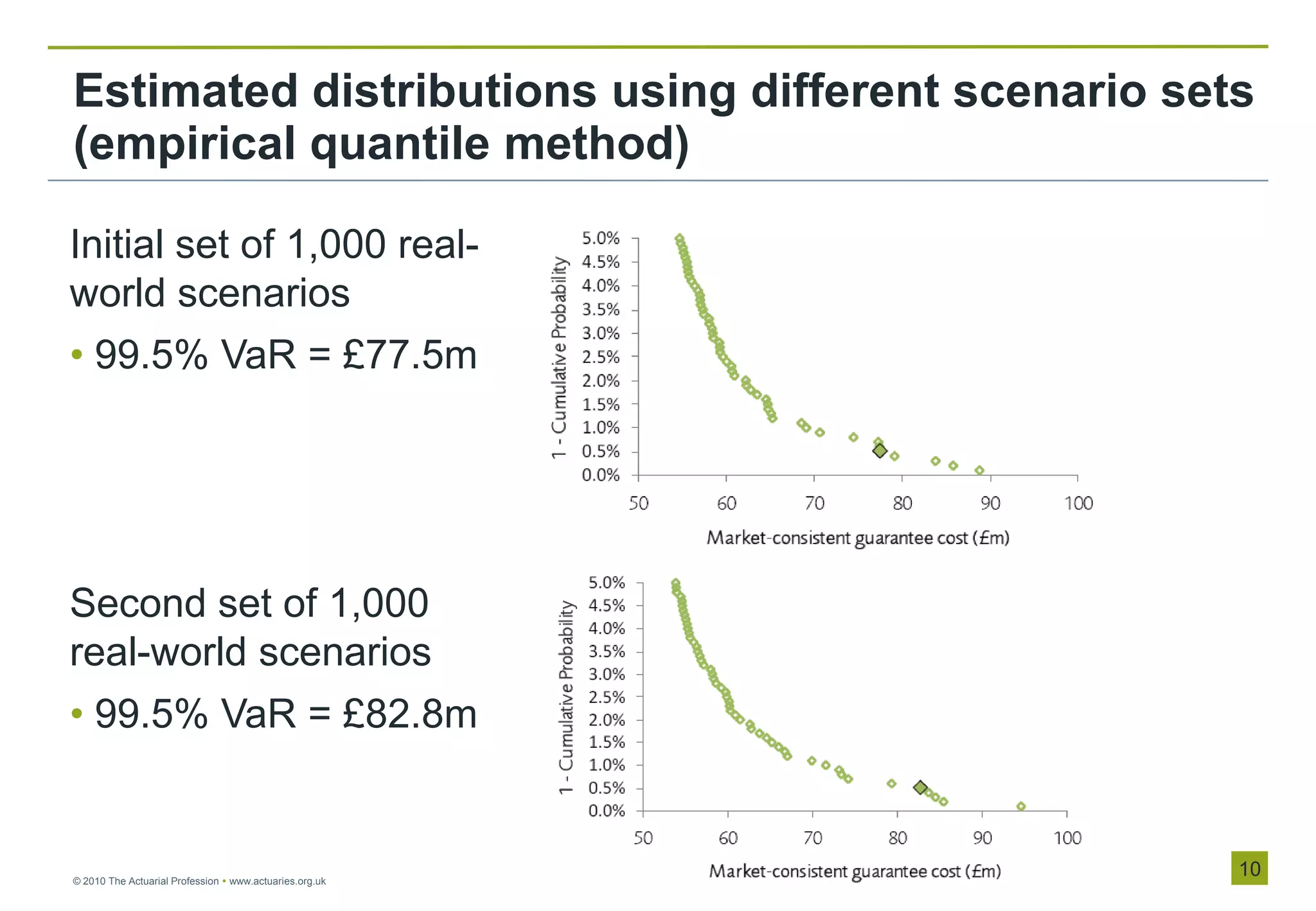
Initial set of 1,000 real-world
scenarios
• 99.5% VaR = £75.9m
• 95% confidence interval =
[71.1m, 84.3m]
Second set of 1,000 real-
world scenarios
• 99.5% VaR = £77.8m
• 95% confidence interval =
[72.2m, 87.7m]
© 2010 The Actuarial Profession www.actuaries.org.uk
15](https://image.slidesharecdn.com/f3part1-13170220924265-phpapp01-110926023050-phpapp01/75/Application-of-Extreme-Value-Theory-to-Risk-Capital-Estimation-16-2048.jpg)