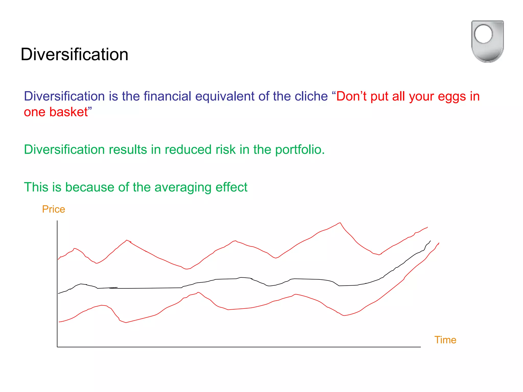
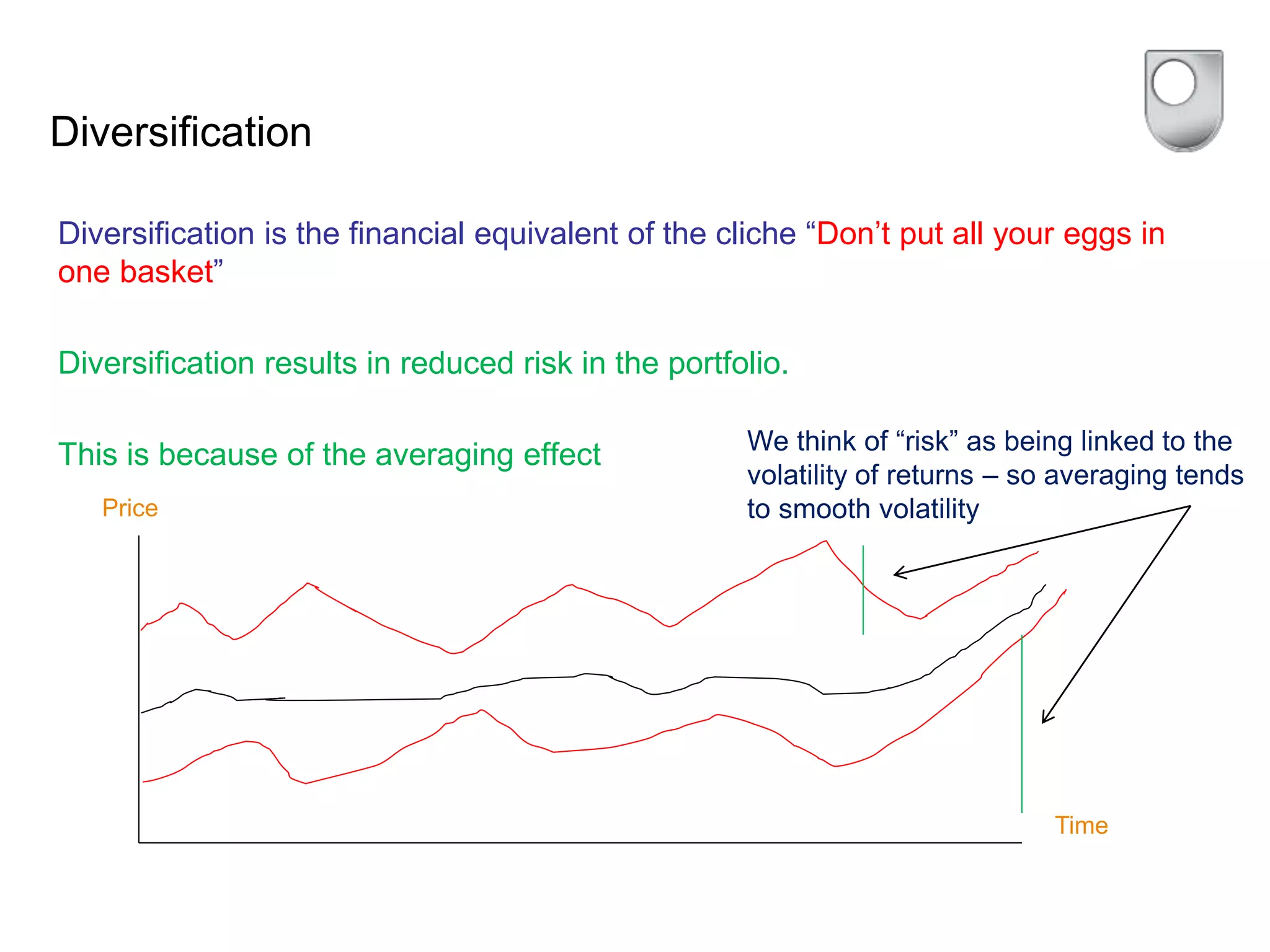
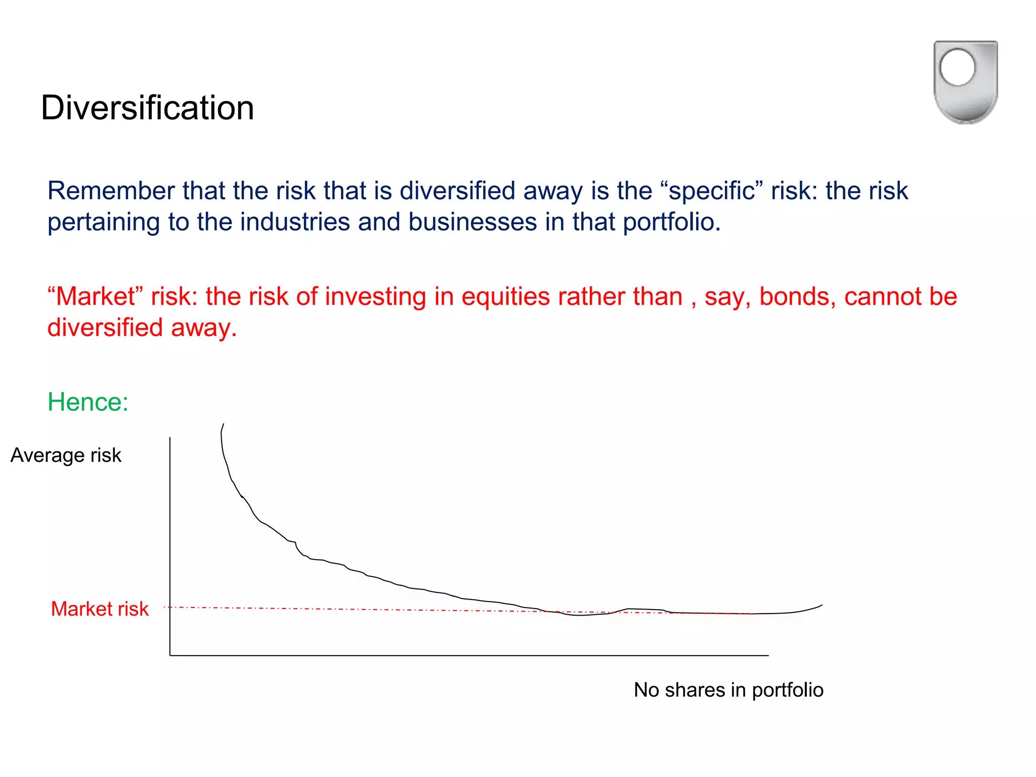
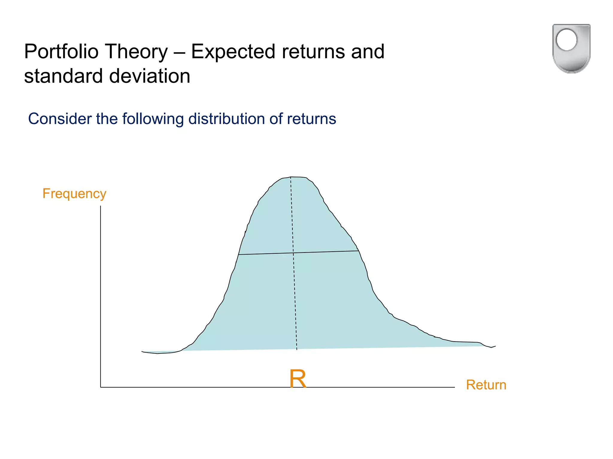
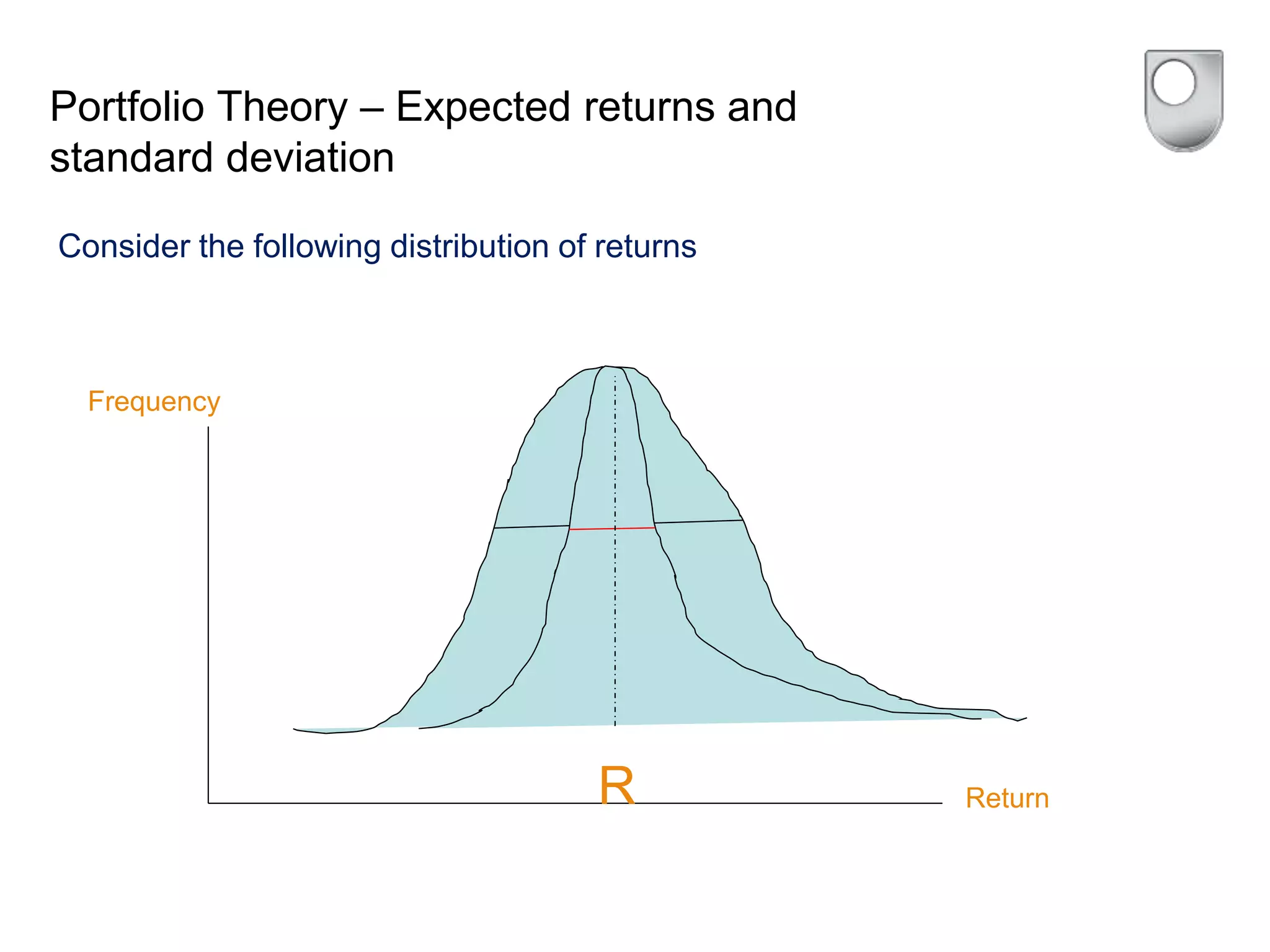
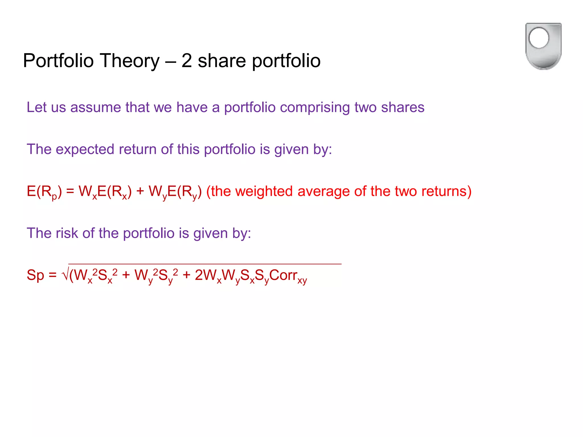
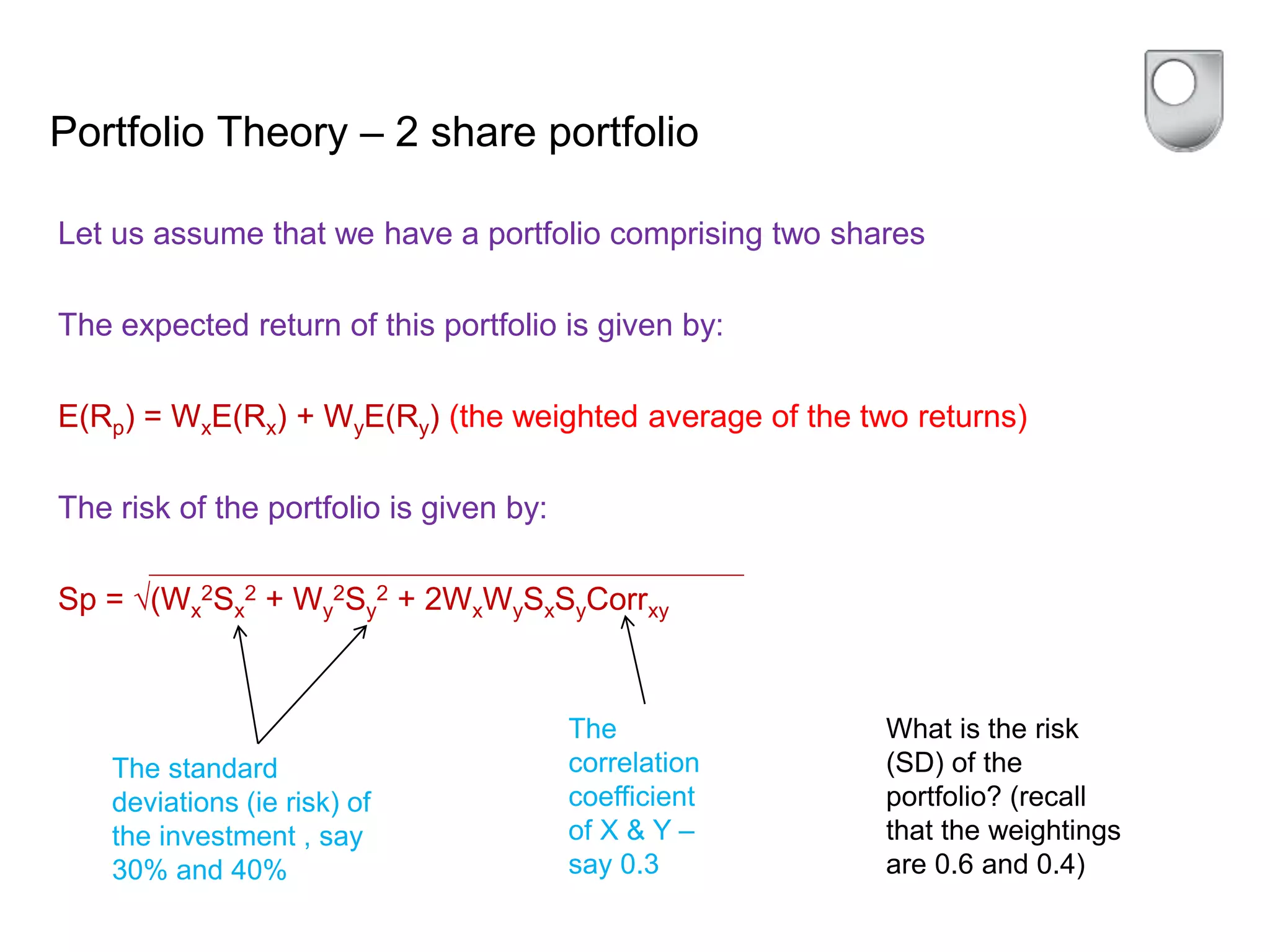
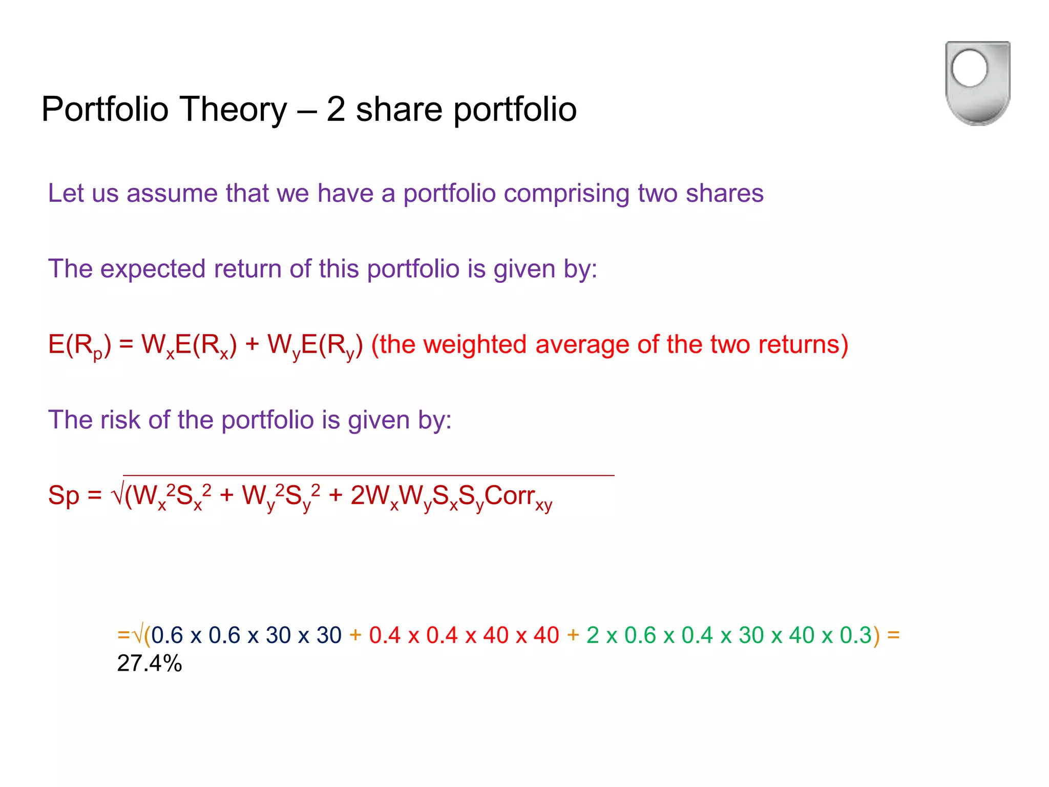
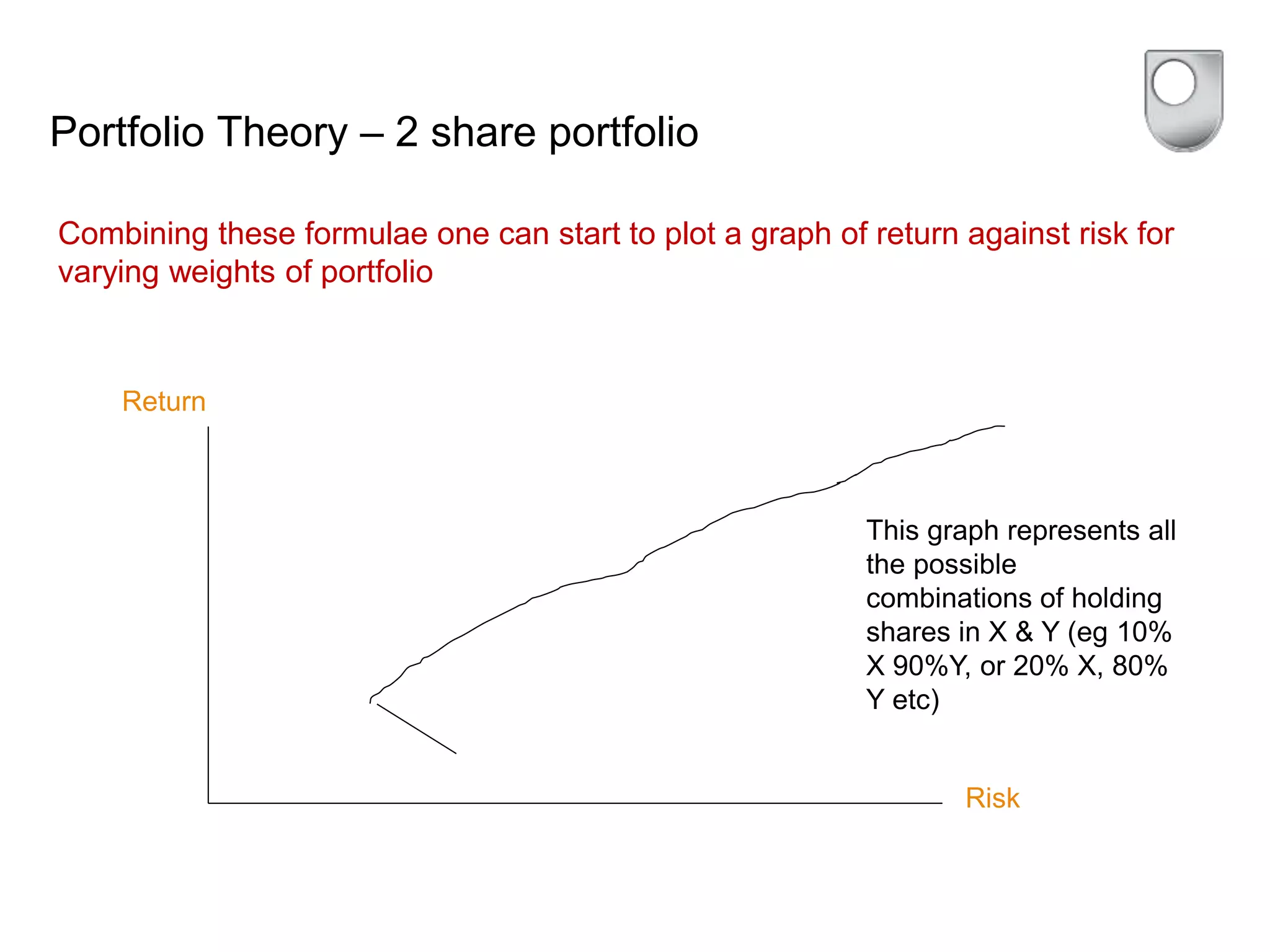
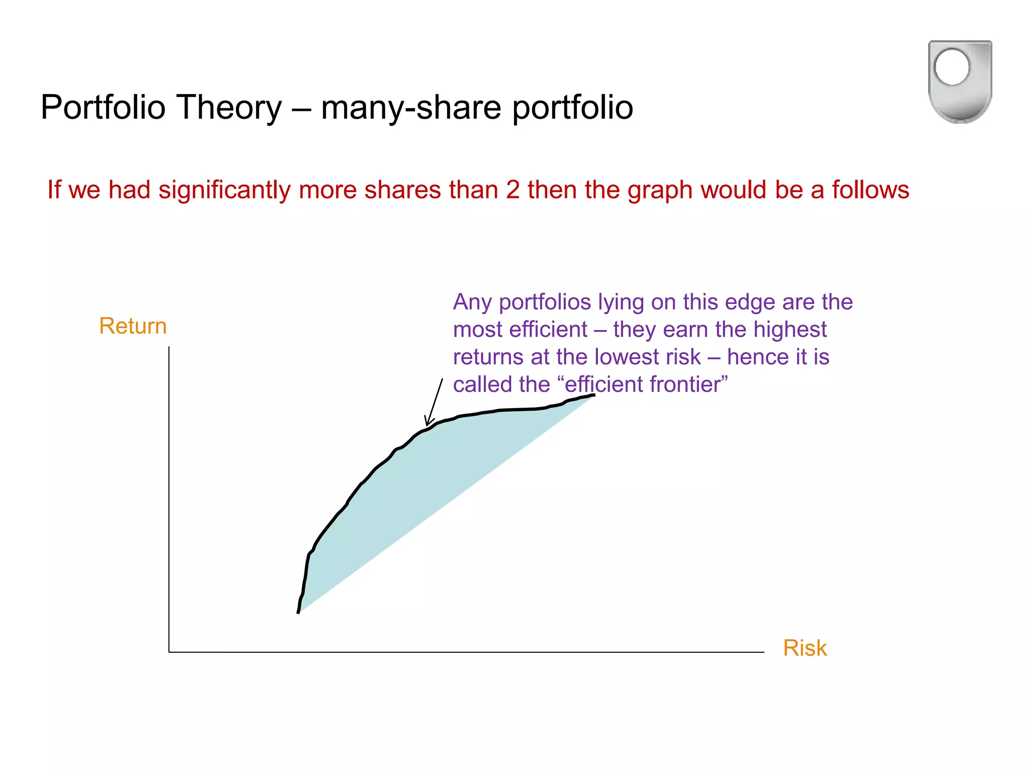
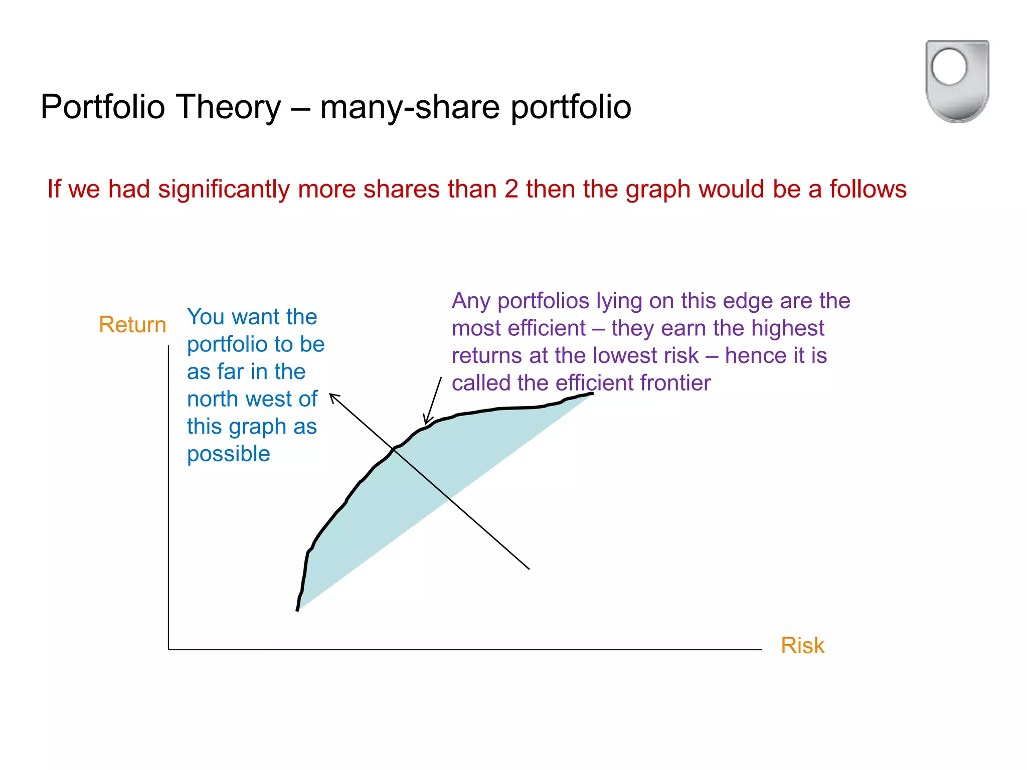
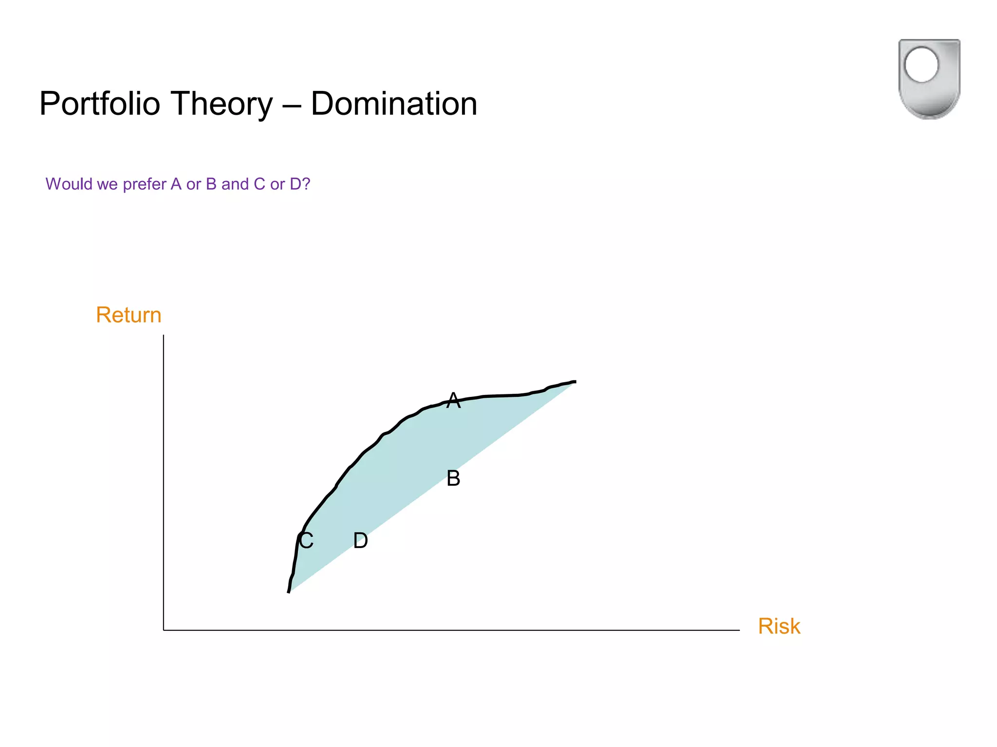
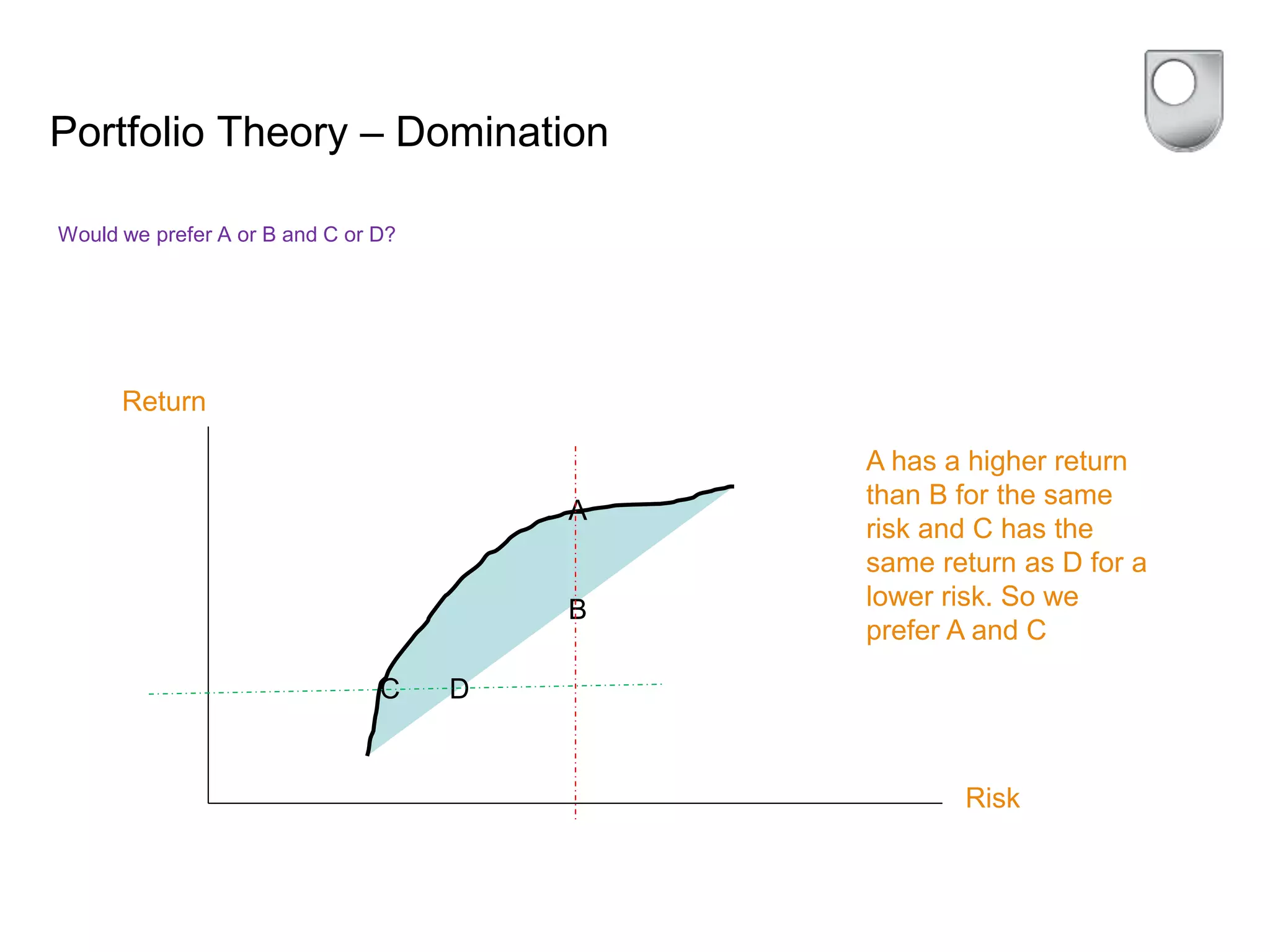
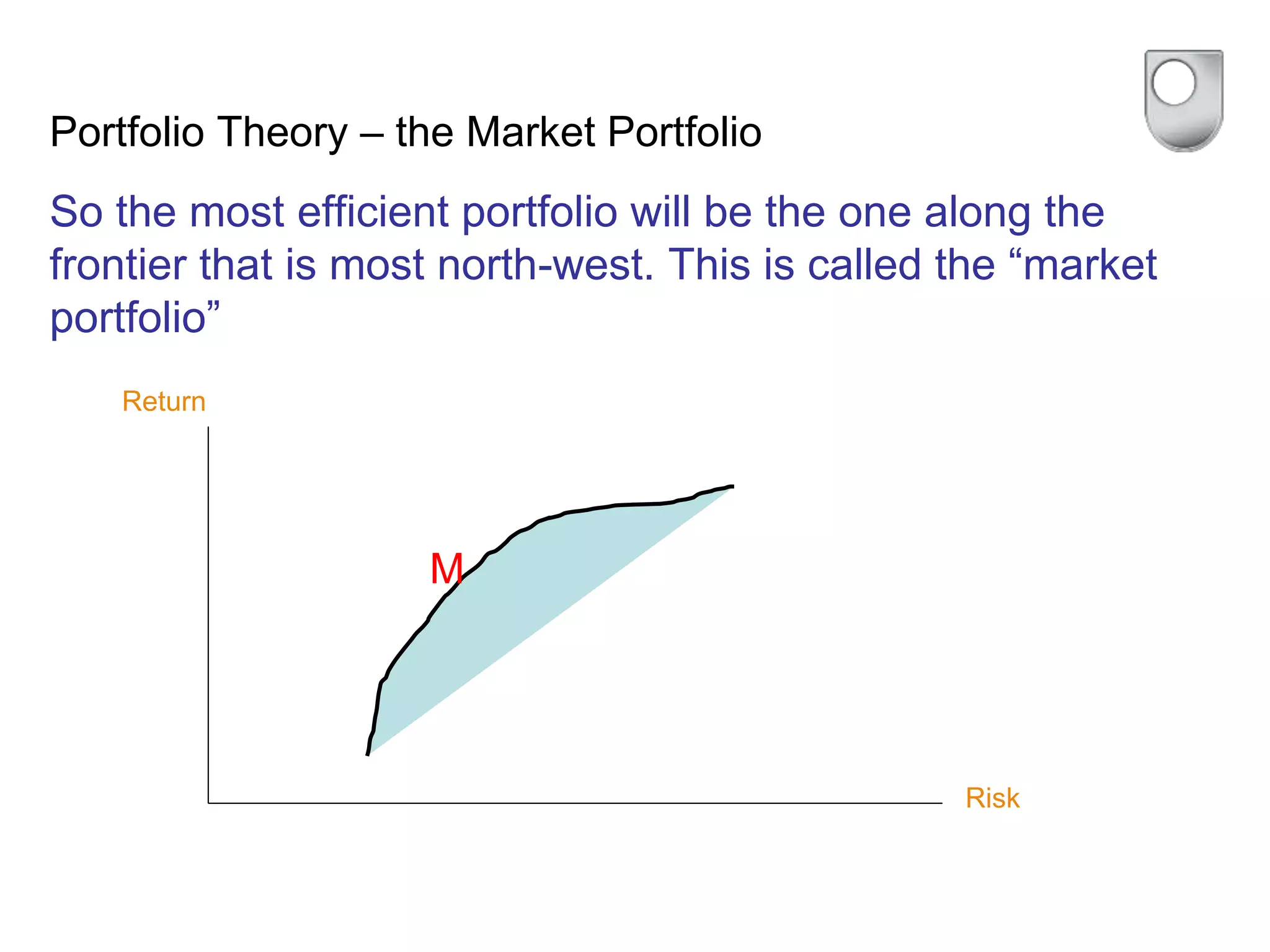
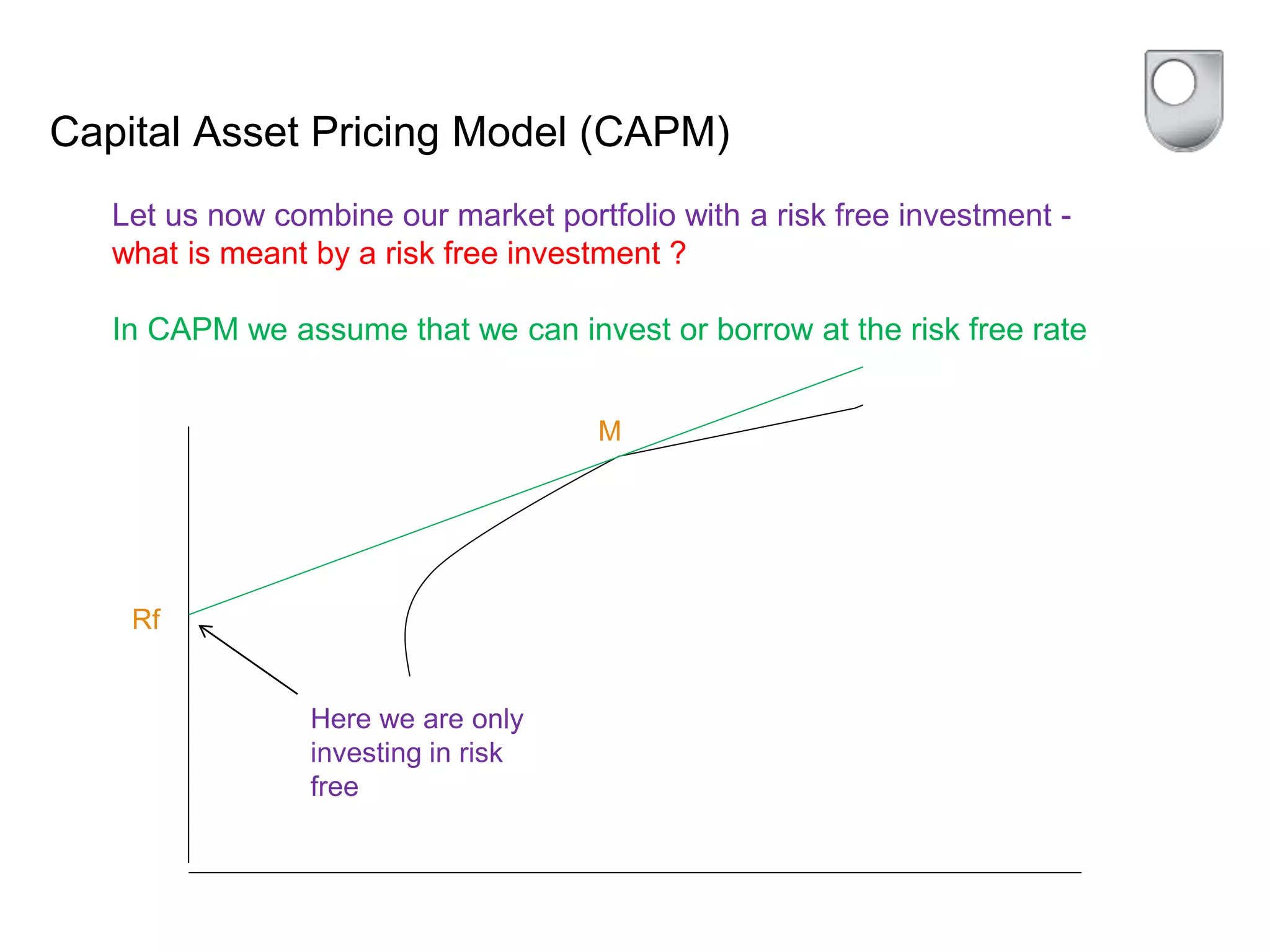
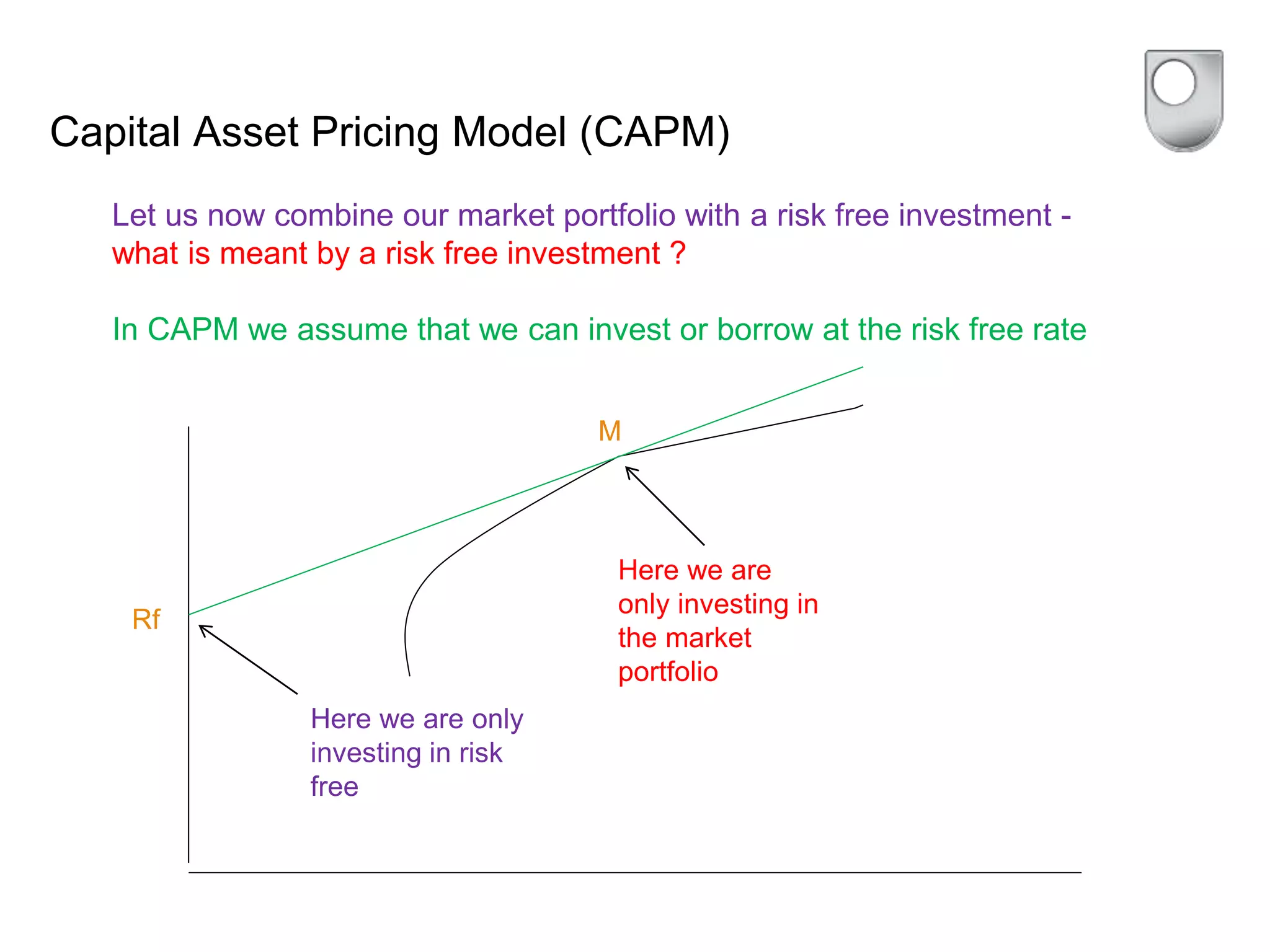
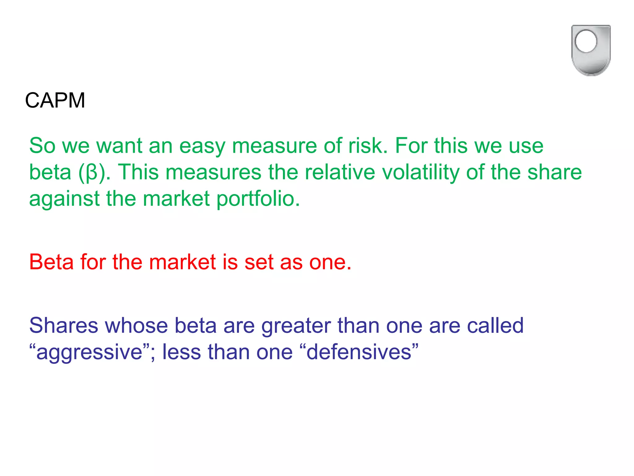
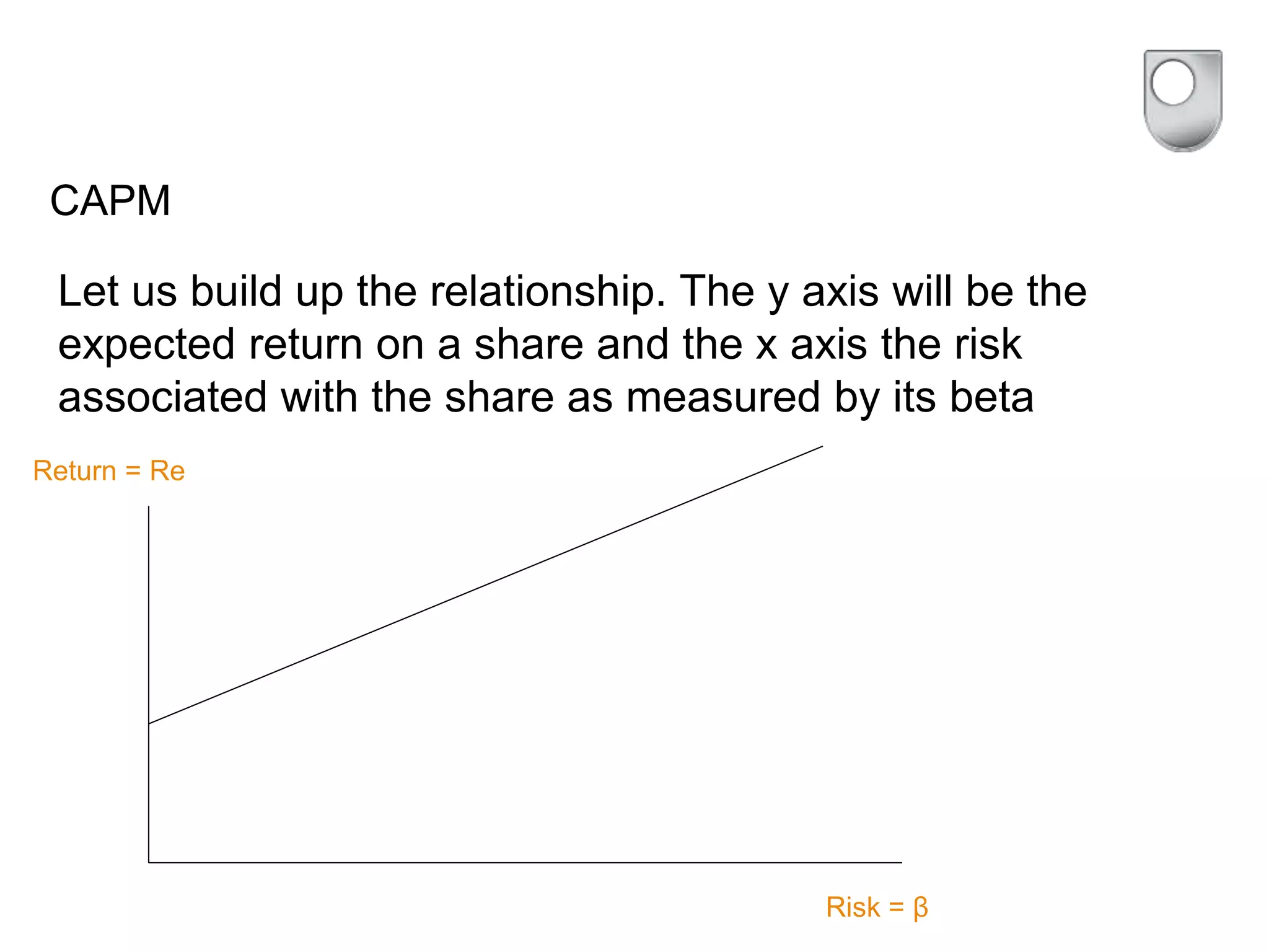
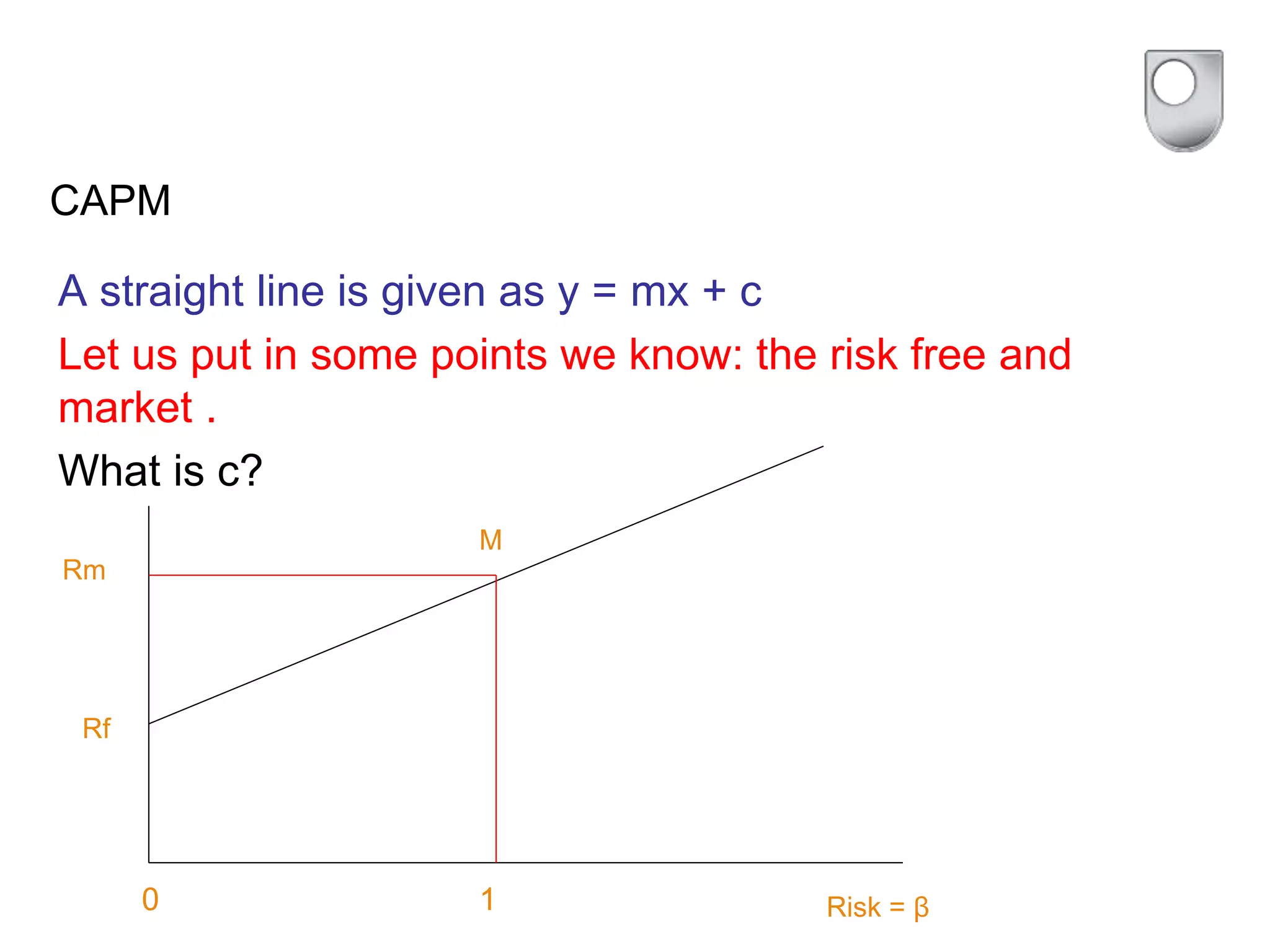
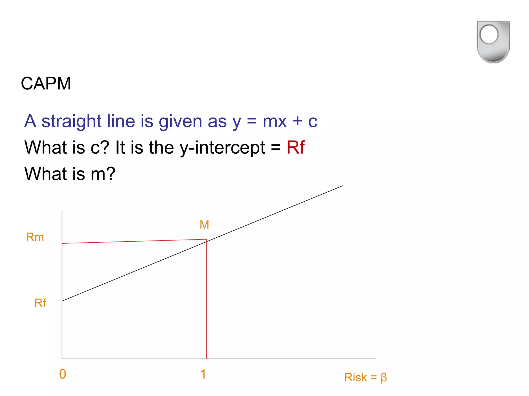
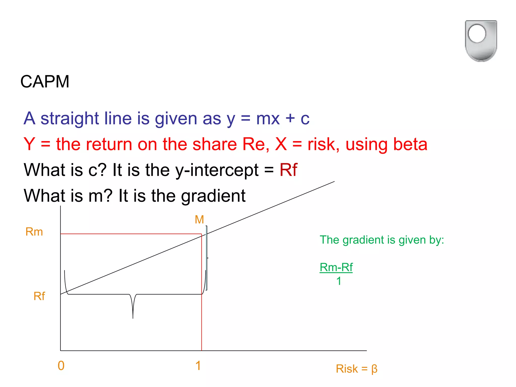
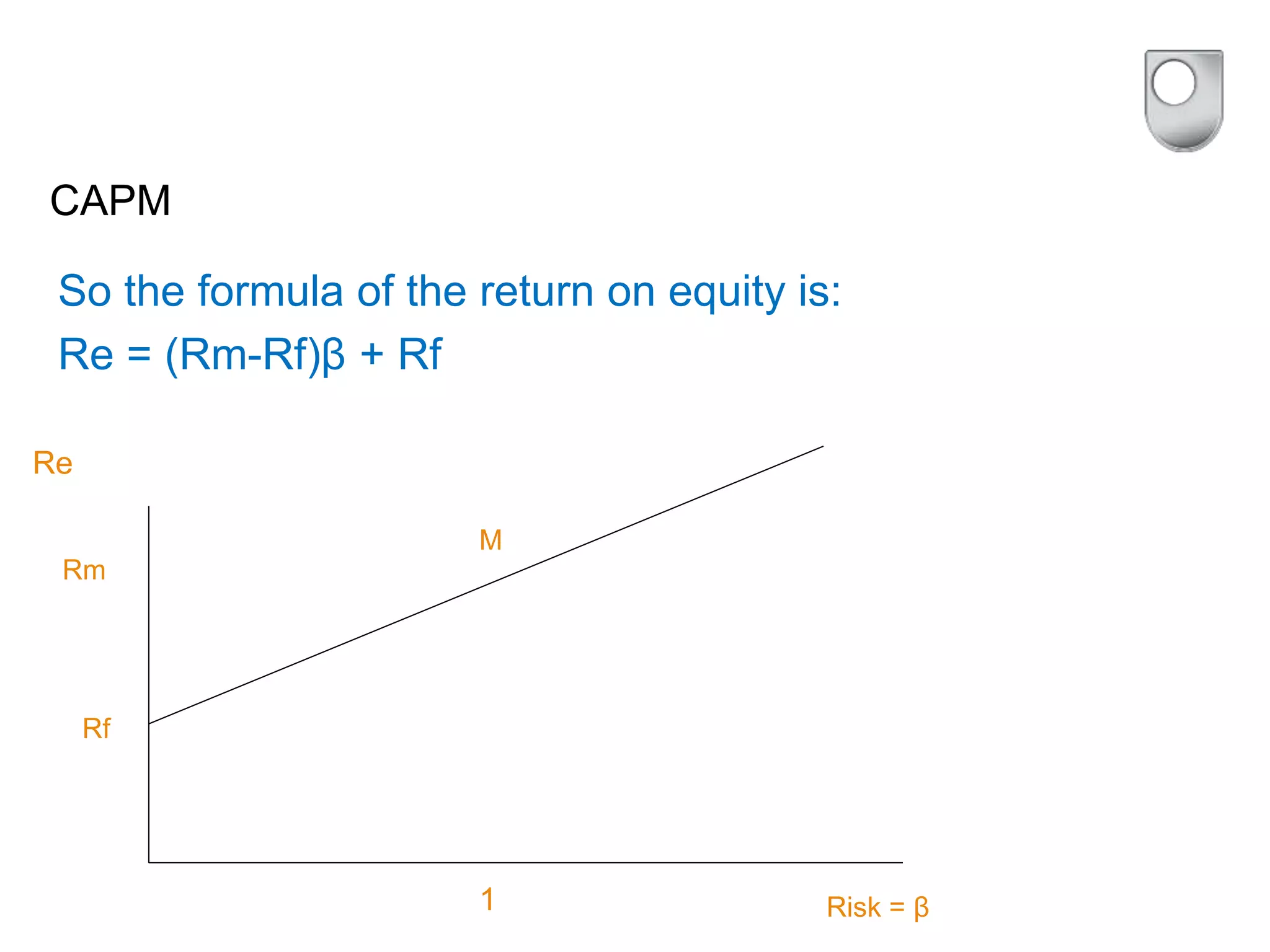
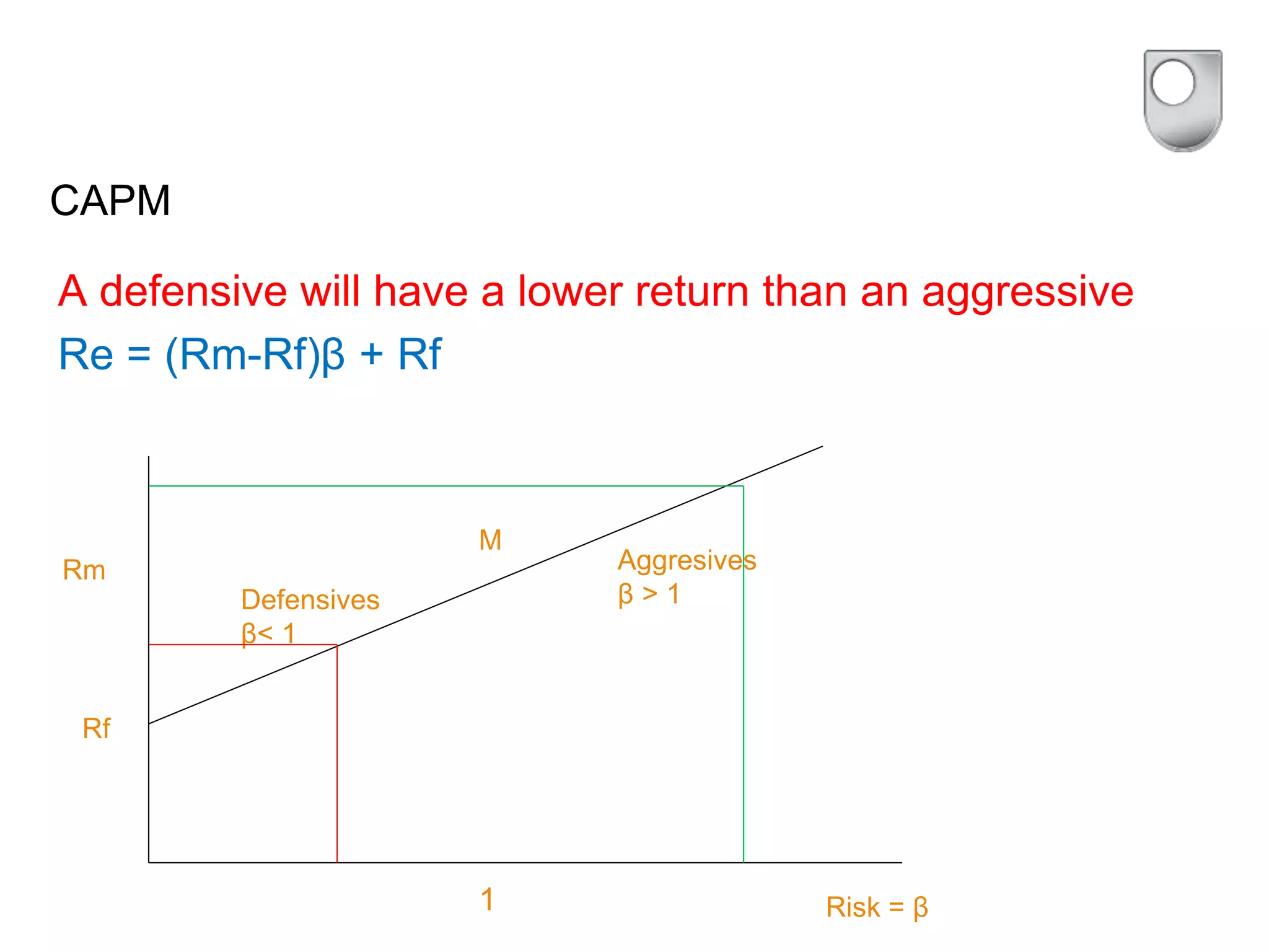
Unit 4
Portfolio Theory and Capital Asset Pricing
Model
Diversification
Diversification is the financial equivalent of the cliche “Don’t put all your eggs in
one basket”
Diversification results in reduced risk in the portfolio.
This is because of the averaging effect
Price
Time
Diversification
Diversification is the financial equivalent of the cliche “Don’t put all your eggs in
one basket”
Diversification results in reduced risk in the portfolio.
This is because of the averaging effect
Price
Time
We think of “risk” as being linked to the
volatility of returns – so averaging tends
to smooth volatility
Diversification
Remember that the risk that is diversified away is the “specific” risk: the risk
pertaining to the industries and businesses in that portfolio.
“Market” risk: the risk of investing in equities rather than , say, bonds, cannot be
diversified away.
Diversification
Remember that the risk that is diversified away is the “specific” risk: the risk
pertaining to the industries and businesses in that portfolio.
“Market” risk: the risk of investing in equities rather than , say, bonds, cannot be
diversified away.
Hence:
Average risk
No shares in portfolio
Market risk
Portfolio Theory
This theory assumes that investors are “risk averse”
Note: “risk averse” does NOT means that investors will not take risks (“risk
avoidance”)
Portfolio Theory
This theory assumes that investors are “risk averse”
Note: “risk averse” does NOT means that investors will not take risks
Instead it means that investors will take on risk if the returns on offer are
sufficient
So the attractions of an investment are a combination of the expected returns
and the risk, as measured by standard deviation
Portfolio Theory – Expected returns and
standard deviation
Consider the following distribution of returns
Frequency
ReturnR
Portfolio Theory – Expected returns and
standard deviation
Consider the following distribution of returns
Frequency
ReturnR
Portfolio Theory – 2 share portfolio
Let us assume that we have a portfolio comprising two shares
The expected return of this portfolio is given by:
E(Rp) = WxE(Rx) + WyE(Ry) (the weighted average of the two returns)
Portfolio Theory – 2 share portfolio
Let us assume that we have a portfolio comprising two shares
The expected return of this portfolio is given by:
E(Rp) = WxE(Rx) + WyE(Ry) (the weighted average of the two returns)
Proportion of the
portfolio that is X
or Y (for example,
0.6 & 0.4)
Expected
returns on X & Y
(eg 10% and
12%)
What is the expected returns here?
Portfolio Theory – 2 share portfolio
Let us assume that we have a portfolio comprising two shares
The expected return of this portfolio is given by:
E(Rp) = WxE(Rx) + WyE(Ry) (the weighted average of the two returns)
Proportion of the
portfolio that is X
or Y (for example,
0.6 & 0.4)
Expected
returns on X & Y
(eg 10% and
12%
Using these figures the expected return
would be 0.6 x 10% + 0.4 x 12% = 10.8%
Portfolio Theory – 2 share portfolio
Let us assume that we have a portfolio comprising two shares
The expected return of this portfolio is given by:
E(Rp) = WxE(Rx) + WyE(Ry) (the weighted average of the two returns)
The risk of the portfolio is given by:
Sp = √(Wx
2Sx
2 + Wy
2Sy
2 + 2WxWySxSyCorrxy
The standard
deviations (ie risk) of
the investment , say
30% and 40%
The
correlation
coefficient
of X & Y –
say 0.3
What is the risk
(SD) of the
portfolio? (recall
that the weightings
are 0.6 and 0.4)
Portfolio Theory – 2 share portfolio
Let us assume that we have a portfolio comprising two shares
The expected return of this portfolio is given by:
E(Rp) = WxE(Rx) + WyE(Ry) (the weighted average of the two returns)
The risk of the portfolio is given by:
Sp = √(Wx
2Sx
2 + Wy
2Sy
2 + 2WxWySxSyCorrxy
=√(0.6 x 0.6 x 30 x 30 + 0.4 x 0.4 x 40 x 40 + 2 x 0.6 x 0.4 x 30 x 40 x 0.3) =
27.4%
Portfolio Theory – 2 share portfolio
Combining these formulae one can start to plot a graph of return against risk for
varying weights of portfolio
Return
Risk
This graph represents all
the possible
combinations of holding
shares in X & Y (eg 10%
X 90%Y, or 20% X, 80%
Y etc)
Portfolio Theory – 2 share portfolio
Combining these formulae one can start to plot a graph of return against risk for
varying weights of portfolio
Return
Risk
You would not pick this
weighting. Why not?
Portfolio Theory – 2 share portfolio
Combining these formulae one can start to plot a graph of return against risk for
varying weights of portfolio
Return
Risk
Because the portfolio at
“A” has the same risk
but a higher return
A
Portfolio Theory – many-share portfolio
If we had significantly more shares than 2 then the graph would be a follows
Return
Risk
Portfolio Theory – many-share portfolio
If we had significantly more shares than 2 then the graph would be a follows
Return
Risk
All of the possible
combinations of the shares
would be in the shaded area
Portfolio Theory – many-share portfolio
If we had significantly more shares than 2 then the graph would be a follows
Return
Risk
Any portfolios lying on this edge are the
most efficient – they earn the highest
returns at the lowest risk – hence it is
called the “efficient frontier”
Portfolio Theory – many-share portfolio
If we had significantly more shares than 2 then the graph would be a follows
Return
Risk
Any portfolios lying on this edge are the
most efficient – they earn the highest
returns at the lowest risk – hence it is
called the efficient frontier
You want the
portfolio to be
as far in the
north west of
this graph as
possible
Portfolio Theory – Domination
Would we prefer A or B and C or D?
Return
Risk
A
C
B
D
Portfolio Theory – Domination
Would we prefer A or B and C or D?
Return
Risk
A
C
B
D
A has a higher return
than B for the same
risk and C has the
same return as D for a
lower risk. So we
prefer A and C
Portfolio Theory – the Market Portfolio
Return
Risk
So the most efficient portfolio will be the one along the
frontier that is most north-west. This is called the “market
portfolio”
M
Capital Asset Pricing Model (CAPM)
Let us now combine our market portfolio with a risk free investment -
what is meant by a risk free investment ?
Capital Asset Pricing Model (CAPM)
Let us now combine our market portfolio with a risk free investment -
what is meant by a risk free investment ?
In CAPM we assume that we can invest or borrow at the risk free rate
Rf
M
Here we are only
investing in risk
free
Capital Asset Pricing Model (CAPM)
Let us now combine our market portfolio with a risk free investment -
what is meant by a risk free investment ?
In CAPM we assume that we can invest or borrow at the risk free rate
Rf
M
Here we are only
investing in risk
free
Here we are
only investing in
the market
portfolio
Capital Asset Pricing Model (CAPM)
Let us now combine our market portfolio with a risk free investment -
what is meant by a risk free investment ?
In CAPM we assume that we can invest or borrow at the risk free rate
Rf
M
Here we are only
investing in risk
free
Here we are
investing in part risk
free and part market
Here we are
only investing in
the market
portfolio
Capital Asset Pricing Model (CAPM)
Let us now combine our market portfolio with a risk free investment -
what is meant by a risk free investment ?
In CAPM we assume that we can invest or borrow at the risk free rate
Rf
M
Here we are only
investing in risk
free
Here we have
BORROWED at the
risk free rate and
invested in the
market portfolio
Here we are
investing in part risk
free and part market
Here we are
only investing in
the market
portfolio
CAPM
As the risk-free – market portfolio relationship is a
straight line it is straightforward to describe it
mathematically.
Once we have that relationship we then have a formula
for the return on a share compared to the risk of that
share
CAPM
So we want an easy measure of risk. For this we use
beta (β). This measures the relative volatility of the share
against the market portfolio.
CAPM
So we want an easy measure of risk. For this we use
beta (β). This measures the relative volatility of the share
against the market portfolio.
Beta for the market is set as one.
Shares whose beta are greater than one are called
“aggressive”; less than one “defensives”
CAPM
Let us build up the relationship. The y axis will be the
expected return on a share and the x axis the risk
associated with the share as measured by its beta
Risk = β
Return = Re
CAPM
A straight line is given as y = mx + c
Let us put in some points we know: the risk free and
market .
What is c?
Rf
M
Risk = β
Rm
10
CAPM
A straight line is given as y = mx + c
What is c? It is the y-intercept = Rf
What is m?
Rf
M
Risk = β
Rm
10
CAPM
A straight line is given as y = mx + c
Y = the return on the share Re, X = risk, using beta
What is c? It is the y-intercept = Rf
What is m? It is the gradient
Rf
M
Risk = β
Rm
1
The gradient is given by:
Rm-Rf
1
0
CAPM
So the formula of the return on equity is:
Re = (Rm-Rf)β + Rf
Rf
M
Risk = β
Rm
1
Re
CAPM
A defensive will have a lower return than an aggressive
Re = (Rm-Rf)β + Rf
Rf
M
Risk = β
Rm
1
Defensives
β< 1
Aggresives
β > 1
Next Time
We shall look at project appraisals – discounted cash
flow etc - from unit 5

Unit4 portfolio theory & CAPM

  • 1.
    Unit 4 Portfolio Theoryand Capital Asset Pricing Model
  • 2.
    Diversification Diversification is thefinancial equivalent of the cliche “Don’t put all your eggs in one basket” Diversification results in reduced risk in the portfolio. This is because of the averaging effect Price Time
  • 3.
    Diversification Diversification is thefinancial equivalent of the cliche “Don’t put all your eggs in one basket” Diversification results in reduced risk in the portfolio. This is because of the averaging effect Price Time We think of “risk” as being linked to the volatility of returns – so averaging tends to smooth volatility
  • 4.
    Diversification Remember that therisk that is diversified away is the “specific” risk: the risk pertaining to the industries and businesses in that portfolio. “Market” risk: the risk of investing in equities rather than , say, bonds, cannot be diversified away.
  • 5.
    Diversification Remember that therisk that is diversified away is the “specific” risk: the risk pertaining to the industries and businesses in that portfolio. “Market” risk: the risk of investing in equities rather than , say, bonds, cannot be diversified away. Hence: Average risk No shares in portfolio Market risk
  • 6.
    Portfolio Theory This theoryassumes that investors are “risk averse” Note: “risk averse” does NOT means that investors will not take risks (“risk avoidance”)
  • 7.
    Portfolio Theory This theoryassumes that investors are “risk averse” Note: “risk averse” does NOT means that investors will not take risks Instead it means that investors will take on risk if the returns on offer are sufficient So the attractions of an investment are a combination of the expected returns and the risk, as measured by standard deviation
  • 8.
    Portfolio Theory –Expected returns and standard deviation Consider the following distribution of returns Frequency ReturnR
  • 9.
    Portfolio Theory –Expected returns and standard deviation Consider the following distribution of returns Frequency ReturnR
  • 10.
    Portfolio Theory –2 share portfolio Let us assume that we have a portfolio comprising two shares The expected return of this portfolio is given by: E(Rp) = WxE(Rx) + WyE(Ry) (the weighted average of the two returns)
  • 11.
    Portfolio Theory –2 share portfolio Let us assume that we have a portfolio comprising two shares The expected return of this portfolio is given by: E(Rp) = WxE(Rx) + WyE(Ry) (the weighted average of the two returns) Proportion of the portfolio that is X or Y (for example, 0.6 & 0.4) Expected returns on X & Y (eg 10% and 12%) What is the expected returns here?
  • 12.
    Portfolio Theory –2 share portfolio Let us assume that we have a portfolio comprising two shares The expected return of this portfolio is given by: E(Rp) = WxE(Rx) + WyE(Ry) (the weighted average of the two returns) Proportion of the portfolio that is X or Y (for example, 0.6 & 0.4) Expected returns on X & Y (eg 10% and 12% Using these figures the expected return would be 0.6 x 10% + 0.4 x 12% = 10.8%
  • 13.
    Portfolio Theory –2 share portfolio Let us assume that we have a portfolio comprising two shares The expected return of this portfolio is given by: E(Rp) = WxE(Rx) + WyE(Ry) (the weighted average of the two returns) The risk of the portfolio is given by: Sp = √(Wx 2Sx 2 + Wy 2Sy 2 + 2WxWySxSyCorrxy
  • 14.
    Portfolio Theory –2 share portfolio Let us assume that we have a portfolio comprising two shares The expected return of this portfolio is given by: E(Rp) = WxE(Rx) + WyE(Ry) (the weighted average of the two returns) The risk of the portfolio is given by: Sp = √(Wx 2Sx 2 + Wy 2Sy 2 + 2WxWySxSyCorrxy The standard deviations (ie risk) of the investment , say 30% and 40% The correlation coefficient of X & Y – say 0.3 What is the risk (SD) of the portfolio? (recall that the weightings are 0.6 and 0.4)
  • 15.
    Portfolio Theory –2 share portfolio Let us assume that we have a portfolio comprising two shares The expected return of this portfolio is given by: E(Rp) = WxE(Rx) + WyE(Ry) (the weighted average of the two returns) The risk of the portfolio is given by: Sp = √(Wx 2Sx 2 + Wy 2Sy 2 + 2WxWySxSyCorrxy =√(0.6 x 0.6 x 30 x 30 + 0.4 x 0.4 x 40 x 40 + 2 x 0.6 x 0.4 x 30 x 40 x 0.3) = 27.4%
  • 16.
    Portfolio Theory –2 share portfolio Combining these formulae one can start to plot a graph of return against risk for varying weights of portfolio Return Risk This graph represents all the possible combinations of holding shares in X & Y (eg 10% X 90%Y, or 20% X, 80% Y etc)
  • 17.
    Portfolio Theory –2 share portfolio Combining these formulae one can start to plot a graph of return against risk for varying weights of portfolio Return Risk You would not pick this weighting. Why not?
  • 18.
    Portfolio Theory –2 share portfolio Combining these formulae one can start to plot a graph of return against risk for varying weights of portfolio Return Risk Because the portfolio at “A” has the same risk but a higher return A
  • 19.
    Portfolio Theory –many-share portfolio If we had significantly more shares than 2 then the graph would be a follows Return Risk
  • 20.
    Portfolio Theory –many-share portfolio If we had significantly more shares than 2 then the graph would be a follows Return Risk All of the possible combinations of the shares would be in the shaded area
  • 21.
    Portfolio Theory –many-share portfolio If we had significantly more shares than 2 then the graph would be a follows Return Risk Any portfolios lying on this edge are the most efficient – they earn the highest returns at the lowest risk – hence it is called the “efficient frontier”
  • 22.
    Portfolio Theory –many-share portfolio If we had significantly more shares than 2 then the graph would be a follows Return Risk Any portfolios lying on this edge are the most efficient – they earn the highest returns at the lowest risk – hence it is called the efficient frontier You want the portfolio to be as far in the north west of this graph as possible
  • 23.
    Portfolio Theory –Domination Would we prefer A or B and C or D? Return Risk A C B D
  • 24.
    Portfolio Theory –Domination Would we prefer A or B and C or D? Return Risk A C B D A has a higher return than B for the same risk and C has the same return as D for a lower risk. So we prefer A and C
  • 25.
    Portfolio Theory –the Market Portfolio Return Risk So the most efficient portfolio will be the one along the frontier that is most north-west. This is called the “market portfolio” M
  • 26.
    Capital Asset PricingModel (CAPM) Let us now combine our market portfolio with a risk free investment - what is meant by a risk free investment ?
  • 27.
    Capital Asset PricingModel (CAPM) Let us now combine our market portfolio with a risk free investment - what is meant by a risk free investment ? In CAPM we assume that we can invest or borrow at the risk free rate Rf M Here we are only investing in risk free
  • 28.
    Capital Asset PricingModel (CAPM) Let us now combine our market portfolio with a risk free investment - what is meant by a risk free investment ? In CAPM we assume that we can invest or borrow at the risk free rate Rf M Here we are only investing in risk free Here we are only investing in the market portfolio
  • 29.
    Capital Asset PricingModel (CAPM) Let us now combine our market portfolio with a risk free investment - what is meant by a risk free investment ? In CAPM we assume that we can invest or borrow at the risk free rate Rf M Here we are only investing in risk free Here we are investing in part risk free and part market Here we are only investing in the market portfolio
  • 30.
    Capital Asset PricingModel (CAPM) Let us now combine our market portfolio with a risk free investment - what is meant by a risk free investment ? In CAPM we assume that we can invest or borrow at the risk free rate Rf M Here we are only investing in risk free Here we have BORROWED at the risk free rate and invested in the market portfolio Here we are investing in part risk free and part market Here we are only investing in the market portfolio
  • 31.
    CAPM As the risk-free– market portfolio relationship is a straight line it is straightforward to describe it mathematically. Once we have that relationship we then have a formula for the return on a share compared to the risk of that share
  • 32.
    CAPM So we wantan easy measure of risk. For this we use beta (β). This measures the relative volatility of the share against the market portfolio.
  • 33.
    CAPM So we wantan easy measure of risk. For this we use beta (β). This measures the relative volatility of the share against the market portfolio. Beta for the market is set as one. Shares whose beta are greater than one are called “aggressive”; less than one “defensives”
  • 34.
    CAPM Let us buildup the relationship. The y axis will be the expected return on a share and the x axis the risk associated with the share as measured by its beta Risk = β Return = Re
  • 35.
    CAPM A straight lineis given as y = mx + c Let us put in some points we know: the risk free and market . What is c? Rf M Risk = β Rm 10
  • 36.
    CAPM A straight lineis given as y = mx + c What is c? It is the y-intercept = Rf What is m? Rf M Risk = β Rm 10
  • 37.
    CAPM A straight lineis given as y = mx + c Y = the return on the share Re, X = risk, using beta What is c? It is the y-intercept = Rf What is m? It is the gradient Rf M Risk = β Rm 1 The gradient is given by: Rm-Rf 1 0
  • 38.
    CAPM So the formulaof the return on equity is: Re = (Rm-Rf)β + Rf Rf M Risk = β Rm 1 Re
  • 39.
    CAPM A defensive willhave a lower return than an aggressive Re = (Rm-Rf)β + Rf Rf M Risk = β Rm 1 Defensives β< 1 Aggresives β > 1
  • 40.
    Next Time We shalllook at project appraisals – discounted cash flow etc - from unit 5