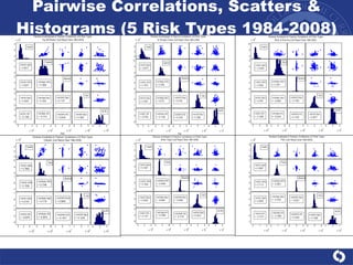
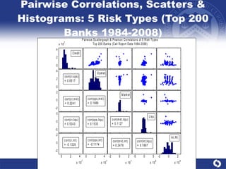
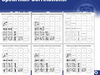
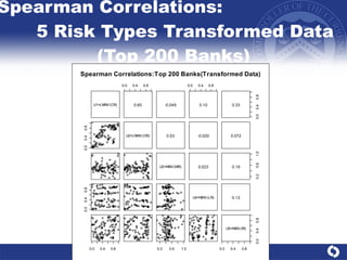
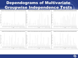
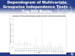
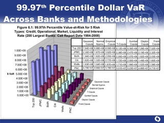
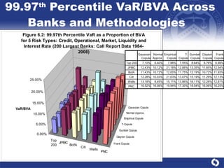
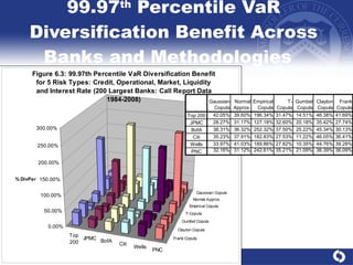
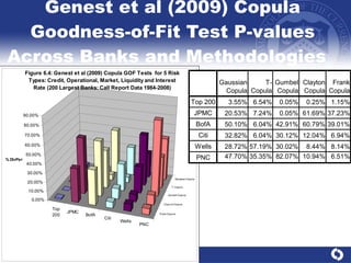
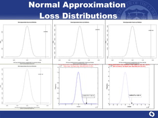
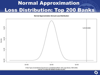
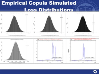
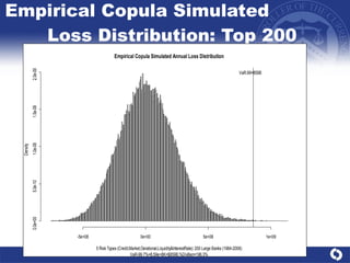
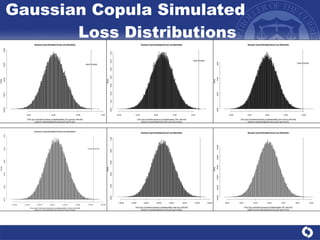
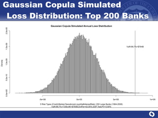
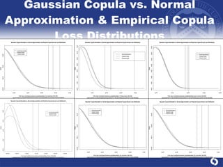
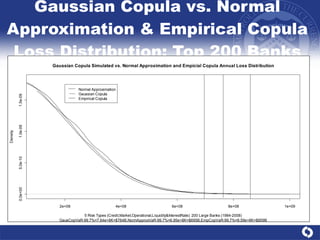
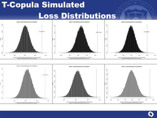
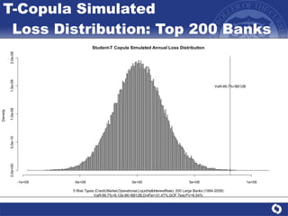
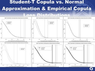
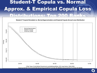
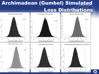
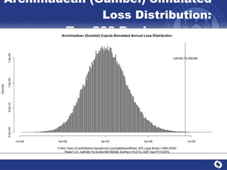
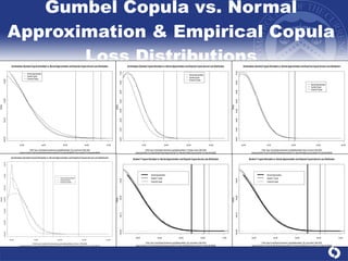
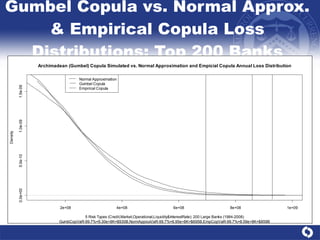
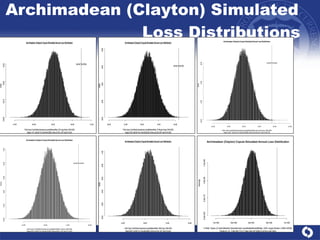
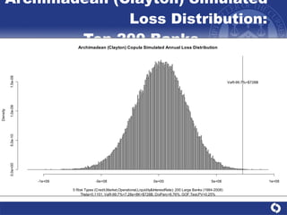
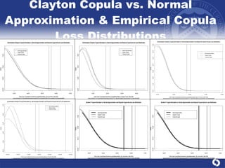
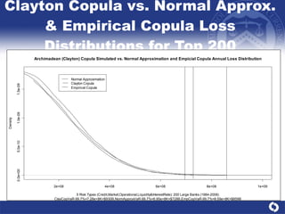
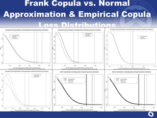
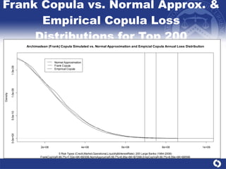
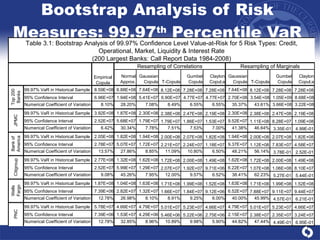
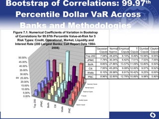
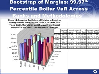
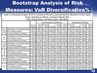
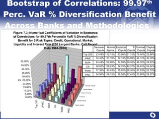
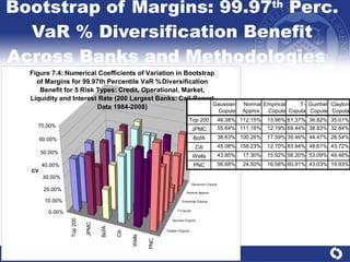
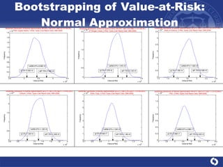
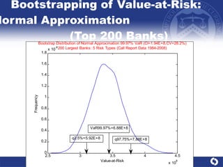
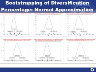
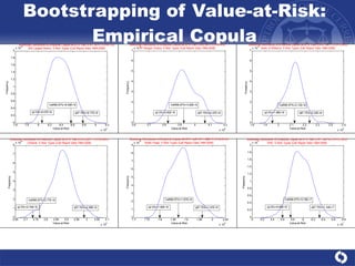
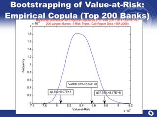
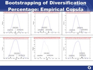
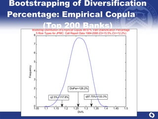
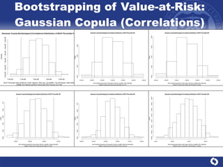
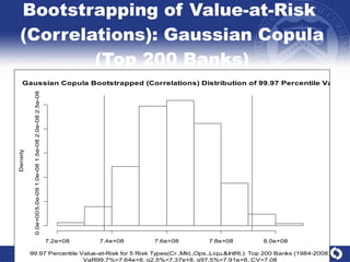
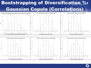
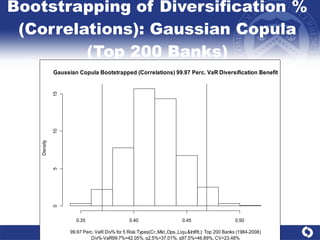
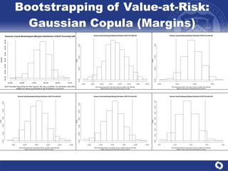
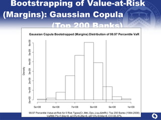
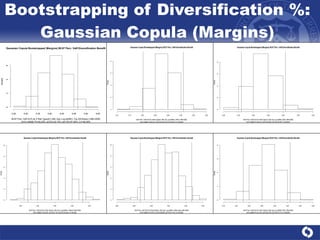
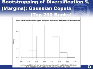
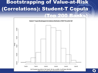
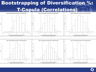
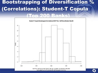
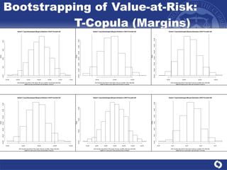
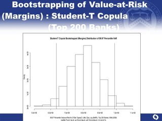
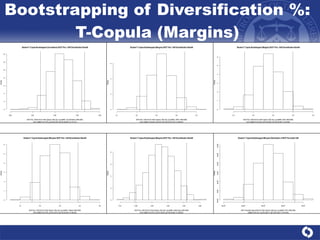
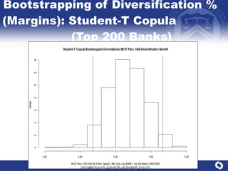
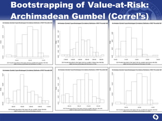
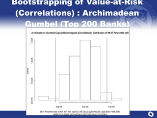
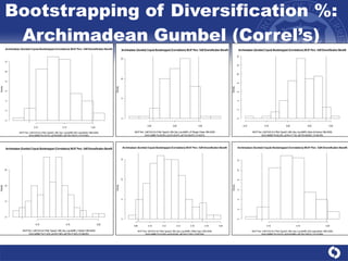
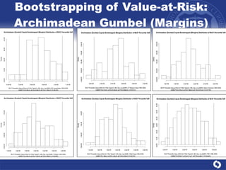
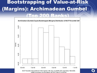
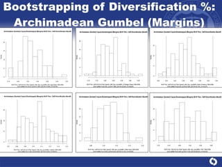
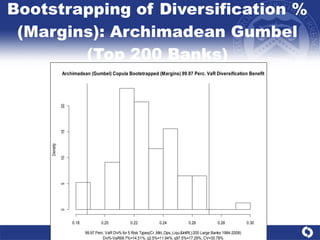
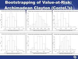
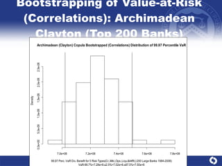
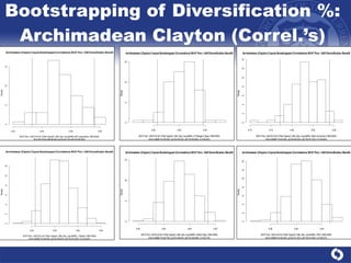
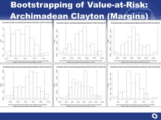
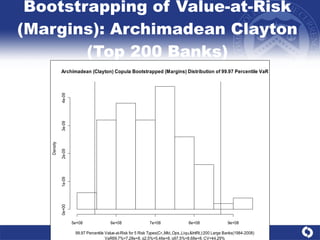
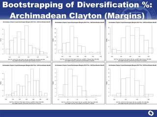
The document summarizes a study on modeling risk aggregation and sensitivity analysis for economic capital at banks. It finds that different risk aggregation methodologies, such as historical bootstrap, normal approximation, and copula models, produce significantly different economic capital estimates ranging from 10% to 60% differences. The empirical copula approach tends to be the most conservative while normal approximation is the least conservative. The results indicate banks should take a conservative approach to quantify integrated risk and consider the impact of methodology choice and parameter uncertainty on economic capital estimates.

1. Models for Risk Aggregation and Sensitivity Analysis: An Application to Bank Economic Capital Hulusi Inanoglu and Michael Jacobs, Jr. Enterprise and Credit Risk Analysis Divisions June 2009 The views expressed herein are those of the authors and do not necessarily represent the views of the Office of the Comptroller of the Currency or the Department of the Treasury.

2. Outline Background and Motivation Introduction and Conclusions Review of the Literature Methodology Data and Summary Statistics Empirical Results Summary and Future Directions

3. Background and Motivation Central challenge to enterprise risk measurement and management faced by diversified financial institutions: a coherent approach to aggregating different risk types. Impetus from rapid financial innovation, evolving supervisory standards (Basel 2) and now recent financial crises Main risks faced (market, credit and operational) have distinct distributional properties & historically modeled differently Extend the scope of the analysis by analyzing A/L mismatch and liquidity risk (Pillar II of IRB framework implications) Utilize actual data representative of major banking institutions’ loss experience (call reports) Explore effect of business mix & inter-risk correlations on total risk Apply copula methods for capturing realistic distributional features of & combining different risk types Compare different copula frameworks (including goodness-of-fit to the data) & evaluate sensitivity to sampling error

4. Background and Motivation (continued) ICAAP: Internal Capital Adequacy Assessment Process Not a model for economic capital (EC), but a bank’s overall framework and mechanism for assessing if EC is appropriate EC may be a quantitative component of ICAAP, but it is not required of all banks by supervisors (only the largest) All banks must perform Stress Testing , which includes analysis around the impact on EC from the following: Scenario Analysis: extreme broad systematic events (or high quantiles of underlying risk factors) Sensitivity Analysis: variation in key parameters due to sampling error or uncertainty or different specifications of the model The contribution of this work is in the latter, as we explore the variability of EC due to underlying statistical noise (sampling error) and to alternative models (specification of copula)

5. Summary and Conclusions Estimated loss distributions for 5 largest banks as of 4Q08 (& Top 200) using quarterly Call Report data 1984-2008 Proxy for 5 risk types with financials: credit (GCO), operational (ONIE), market (4QDNTR), liquidity (4QDLGD) & interest income (4QDIG) Different risk aggregation methodologies: historical bootstrap (empirical copula), Normal approx., Copulas (Gaussian,Student-t,Archimadean) Empirical copula (normal approx.) is found to be most (least) conservative (contrary to asymptotics) & most (least) stable in bootstrap experiment vs. standard copula methods But EC implies significantly greater proportional diversification benefits Document significant differences across banks & aggregation methodologies in absolute risk measures & diversification benefits (ranging 10% to 60%) Simple addition over-states risk relative to standard copula formulations by about 30%-20%

6. Summary and Conclusions (continued) Goodness-of-fits tests are mixed across copula models, but in many cases show evidence of poor fit to the data Fail to find the effect of business mix to exert a directionally consistent an impact on total integrated diversification benefits In a bootstrapping experiment, find the variability of the VaR to be significantly lower (higher) for the empirical & Gaussian copula than other formulations (Normal approximation) Find that the contribution of the sampling error in the parameters of the marginal distributions to be an order or magnitude greater than that or the correlation matrices. Results constitute a sensitivity analysis that argues for practitioners to err on the side of conservatism in considering a non-parametric EC approach to quantify integrated risk .

7. Review of the Literature Sklar (1956): mathematical foundation of copula methodology Existence of a copula to connect any set of marginal distributions Embrechts (1999, 2002): first applications to risk management Li (2000): credit risk management Frey & McNeil (2001): copulas as a generalization of dependence according to linear correlations Motivation for applying the technique to understanding tail events Poon (2001): alternative of a data intensive multivariate extension of extreme value theory (need joint tail events) Most finance applications in portfolio risk measurement: Bouye (2001), Longin and Solnik (2001) and Glasserman et al (2002) Embrechts et al (2003): reviews & extends recent results on distributional bounds for functions of dependent risks Main emphasis on Value-at-Risk as a risk measure Ward and Lee (2002): joint loss distributions (pair-wise roll-ups Gaussian copula marginal distributions) analytical & numerical Kuritzkes et al. (2003): financial conglomerate & Gaussian copula for a large set of diversification results

8. Review of the Literature (continued) Dimakos and Aas (2004): bank with life insurance subsidiary (risk = conditional marginal + unconditional credit risk) Imposing conditional independence through set of sufficient conditions such that only pair-wise dependence remains Schuermann & Rosenberg (2006): integrated risk management for typical large, internationally active financial institution Copula approach for aggregating 3 main risk types (market, credit & operational) where the distributional properties varies widely Impact of business mix and inter-risk correlations on total risk: former found more important (“good news” for supervisors) Compare various simplified approaches applied by practitioners (variance-covariance approach & regulatory addition approach) Aas (2007): incorporates ownership risk from a life insurance subsidiary & combines a base-& top-level aggregation Risk factors: multivariate GARCH model with Student-t errors The model, originally developed DnB Nor is adapted to of Basel II Genest et al (2009): reviews literature on goodness-of-fit tests for copula models and proposes a “blanket” test with good size/power properties

9. Methodology: Value-at-Risk Consider a single-valued function (simple sum of losses) of the risk factors (dollar losses: e.g., P&L, credit losses) from time t to t + Δ (Δ = horizon): The Value-at-Risk at the confidence level α between times t and t + Δ (Δ is the horizon) is related to the α th quantile of F( π ( X)) as and denoted by: Vector of K risk factors at time t having a joint distribution function. Serious issues with VaR: coherence (Artzner 1997, 1999), loss of information vs. focusing on entire distribution (Diebold et al,1998; Christoffersen and Diebold, 2000; Berkowitz, 2001), possibility for unbounded concentration risk & “gaming” (Embrechts et al. 1999, 2002). Therefore, we also look at the expected shortfall (ES), measuring expectation of the risk exposure conditional upon exceeding a VaR threshold:

10. Value-at-Risk: The Variance-Covariance Approximation Note simply summing losses so no portfolio weights so that standard deviation of horizon losses is the root of the simple quadratic form: Interesting & ubiquitous special case (motivated by Markowitz (1959) investment theory), seen in many practical EC frameworks (HSBC, 2008), where risk factors have a valid variance-covariance matrix & are multivariate Gaussian (or risk managers/investors do not care about moments > 2 nd ) : Under the assumptions that minimizing the variance of the total loss is the object, NVaR (N=“normal”) is proportional to the standard deviation of the position according to the quantile of the standard normal distribution: Case in which the standardized distribution of the positions is the same as that of the total loss yields “Hybrid Value-at-Risk” (HVaR) as follows

11. Value-at-Risk: The Variance-Covariance Approximation (continued) The case in which we assume risk factors or losses to be perfectly correlated we call “Perfectly-correlated Value-at-Risk” (PVaR): The case in which we assume risk factors or losses to be uncorrelated we call “Uncorrelated Value-at-Risk” (UVaR): Obviously that in this framework and in a “mean-variance world”, PVaR (UVaR) forms an upper (lower) bound on the HVaR measure of risk:

12. Methodology: The Method of Copulas If the joint distribution is continuously differentiable to the k th degree, that is sufficient for the copula to exist and be unique Frechet-Hoeffding boundaries for copulas: minimum (maximum) copula, the case of perfect inverse (positive) dependence amongst random variables: Fundamental result (Sklar, 1956): under the appropriate & general mathematical regularity conditions) any joint distribution can be expressed in terms of a copula (or dependence) function & set of marginal distributions. If we have a K-vector of risk factors, then a copula is a multivariate joint distribution defined on the K-dimensional unit cube, such that each marginal distribution is uniformly distributed on the unit interval: . Four technical conditions sufficient for a copula to exist (Nelson, 1999):

13. Methodology: The Method of Copulas (continued) Note that P is not necessarily the correlation matrix of X , but in this context the Spearman rank-order correlations of the transformed variables (in cases of other copulas this may a different dependence measure of dependence) While for a random vector having a valid joint distribution function the copula will always exist, there is no guarantee that it will be unique. May always construct a copula for any multivariate distribution according to the method of inversion Intuitively: removing the effects of the marginal distributions on dependence relation by substituting in the marginal quantile functions in lieu of the arguments to the original distribution function If we have a random vector in the k th hyper-unit, them we may write the copula as a function as this as follows: Consider a rather common choice of copula function, the Gaussian copula , simply a multivariate standard normal distribution with covariance matrix P :

14. Methodology: The Method of Copulas (continued) Computationally equivalent to historical simulation method of simply resampling the observed history of joint losses with replacement (or bootstrapping) Historically, this was on of the standard method for computing VaR for trading positions amongst market risk department practitioners. Another commonly employed and closely related choice of copula in the elliptical family is the t-copula with degrees-of-freedom ν : Often neglected but fundamental & interesting: empirical copula , a useful tool where there is high uncertainty on the underlying data distribution Procedure: transform the empirical data distribution into an "empirical copula" by warping such that the marginal distributions become uniform Mathematically the empirical copula frequency function has the following representation:

15. Methodology: The Method of Copulas (continued) Where the generator function is indexed by a parameter θ , a whole family of copulas may be Archimedean, as in the Clayton copula : An important class of copulas: Archimadean family , having simple forms with properties (e.g., associativity) & a variety of dependence structures Unlike elliptical copulas, most have closed-form solutions and are not derived from the multivariate distribution functions using Sklar’s Theorem One particularly simple form of k-dimensional Archimadean copula having generator function (satisfying certain conditions) : Several special cases of note. In the product (independent) copula there is no dependence between variates (i.e., density function is unity everywhere): Where parameter θ =0 we have the case of statistical independence The Clayton copula exhibits negative tail dependence

16. Methodology: The Method of Copulas (continued) Another commonly employed copulas in the Archimadean family include the Gumbel copula (having the property of positive tail dependence ): Finally, we consider the Frank copula (having the property of neither positive nor negative tail dependence ): We may simulate realizations from a multivariate distribution by generating independent random vectors For example, in the Gaussian case, it is either standard normal and independent random variables that we generate With knowledge of the marginal distributions of the risk factors (which can be estimated either parametrically or non-parametrically), we can derive a rank-order correlation matrix of the transformed marginal data We can make our independent random vectors correlated (by means of a Cholesky decomposition, for instance)

17. Data Description Quarterly call report data for top 200 banks 1Q84-4Q08 Corrected for mergers & acquisitions: legacy banks synthetically added into currently surviving banks on pro forma basis Proxy for 5 risk types using financial statement data Credit Risk (CR): gross charge-offs (“GCO”) Operational Risk (OR): total other non-interest expense (“ONIE”) Market Risk (MR): (minus of) net trading revenues deviation from moving 4 quarter moving average (“NTR-4QD”) Liquidity Risk (LR): liquidity gap (total loans minus total deposits) deviation from 4 quarter moving average (“LR-4QD”) Interest Rate Risk (IR): interest rate gap (interest expense on deposits minus interest income on loans) deviation from 4 quarter moving average (“IRG-4QD”)

18. Empirical Results: Summary Statistics (Call Report Data)

19. Empirical Results: Summary Statistics (Call Reports & CRSP)

20. Empirical Results: Summary Statistics (Call Report Variables)

21. Empirical Results: Summary Statistics (Call Report & CRSP)

22. Empirical Results: Summary Statistics (Risk Proxies)

23. Historical Quarterly Risk Proxies: Loss Distributions (1984-2008)

24. Historical Quarterly Risk Proxies: Loss Distributions (Top 200 Banks 1984-2008)

25. Historical Quarterly Risk Proxies: Time Series (1984-2008)

26. Historical Quarterly Risk Proxies: Time Series (Top 200 Banks 1984-2008)

27. Pairwise Correlations: Pearson vs. Spearman (5 Risk Types 1984-2008)

28. Pairwise Correlations, Scatters & Histograms (5 Risk Types 1984-2008)

29. Pairwise Correlations, Scatters & Histograms: 5 Risk Types (Top 200 Banks 1984-2008)

30. Spearman Correlations: 5 Risk Types Transformed Data

31. Spearman Correlations: 5 Risk Types Transformed Data (Top 200 Banks)

32. Dependograms of Multivariate Groupwise Independence Tests

33. Dependogram of Multivariate Groupwise Independence Tests – Top 200 Banks

34. Multivariate Groupwise Independence Tests: P-Values

35. Alternative Risk Measures: 99.97 th Percentile VaR

36. 99.97 th Percentile Dollar VaR Across Banks and Methodologies

37. 99.97 th Percentile VaR/BVA Across Banks and Methodologies

38. 99.97 th Percentile VaR Diversification Benefit Across Banks and Methodologies

39. Genest et al (2009) Copula Goodness-of-Fit Test P-values Across Banks and Methodologies

40. Discussion of 99.97 th Percentile VaR and % Diversification Benefit & GOF Tests of Model Fit Dollar VaR (VaR/BVA) increases montonically (generally decreases) with size of the institution VCA (ECS or the AGCS) produces consistently the lowest (highest) VaR; TCS in follows in conservativeness, while the GCS & AFCS (ACCS) is usually toward the middle (low side) ECS yields highest PDBs (127%-252%) vs. other models (10%-50%); GCS tends to lie in the middle (41-58%), VCA to the lower end (31-41%) & GCAS is the lowest (10-21%) No directionally consistent pattern in PDBs across different business mixes (i.e., higher % trading vs. lending assets) GOF tests highly mixed (reject null 14/30 cases), no pattern, not at very high levels of significance->models generally OK?

41. Alternative Risk Measures: 99 th Percentile Expected Shortfall

42. Normal Approximation Loss Distributions

43. Normal Approximation Loss Distribution: Top 200 Banks

44. Empirical Copula Simulated Loss Distributions

45. Empirical Copula Simulated Loss Distribution: Top 200

46. Gaussian Copula Simulated Loss Distributions

47. Gaussian Copula Simulated Loss Distribution: Top 200 Banks

48. Gaussian Copula vs. Normal Approximation & Empirical Copula Loss Distributions

49. Gaussian Copula vs. Normal Approximation & Empirical Copula Loss Distribution: Top 200 Banks

50. T-Copula Simulated Loss Distributions

51. T-Copula Simulated Loss Distribution: Top 200 Banks

52. Student-T Copula vs. Normal Approximation & Empirical Copula Loss Distributions

53. Student-T Copula vs. Normal Approx. & Empirical Copula Loss Distributions: Top 200 Banks

54. Archimadean (Gumbel) Simulated Loss Distributions

55. Archimadean (Gumbel) Simulated Loss Distribution: Top 200 Banks

56. Gumbel Copula vs. Normal Approximation & Empirical Copula Loss Distributions

57. Gumbel Copula vs. Normal Approx. & Empirical Copula Loss Distributions: Top 200 Banks

58. Archimadean (Clayton) Simulated Loss Distributions

59. Archimadean (Clayton) Simulated Loss Distribution: Top 200 Banks

60. Clayton Copula vs. Normal Approximation & Empirical Copula Loss Distributions

61. Clayton Copula vs. Normal Approx. & Empirical Copula Loss Distributions for Top 200

62. Archimadean (Frank) Simulated Loss Distributions

63. Archimadean (Frank) Simulated Loss Distribution: Top 200 Banks

64. Frank Copula vs. Normal Approximation & Empirical Copula Loss Distributions

65. Frank Copula vs. Normal Approx. & Empirical Copula Loss Distributions for Top 200

66. Bootstrap Analysis of Risk Measures: 99.97 th Percentile VaR

67. Bootstrap of Correlations: 99.97 th Percentile Dollar VaR Across Banks and Methodologies

68. Bootstrap of Margins: 99.97 th Percentile Dollar VaR Across Banks and Methodologies

69. Bootstrap Analysis of Risk Measures: VaR Diversification%

70. Bootstrap of Correlations: 99.97 th Perc. VaR % Diversification Benefit Across Banks and Methodologies

71. Bootstrap of Margins: 99.97 th Perc. VaR % Diversification Benefit Across Banks and Methodologies

72. Discussion: Bootstrap of 99.97 th Perc. VaR & % Diver. Benefit Across Banks and Methodologies We fail to observe a consistent pattern in the variability of VaR or PDB across size or types of banks (i.e., business mix). For either the bootstrap of margins or correlations for VaR or PDB, ECS (VCA) yields lowest (highest) NCVs Across models or banks NCVs are an order of magnitude higher for the resampling of margins vs. correlations This difference is accentuated for VaR vs. PDB. NCVs are higher for the PDB vs. VaR: excluding ECS, NCVs for VaR in bootstrap of correlations (margins) range in 5.9%-32.8% (25.2%-56.1%); respective PDB numbers are 17.3%-158.2% (19.9%-83.9%) .,..

73. Bootstrapping of Value-at-Risk: Normal Approximation

74. Bootstrapping of Value-at-Risk: Normal Approximation (Top 200 Banks)

75. Bootstrapping of Diversification Percentage: Normal Approximation

76. Bootstrapping of Diversification Percentage: Normal Approximation (Top 200 Banks)

77. Bootstrapping of Value-at-Risk: Empirical Copula

78. Bootstrapping of Value-at-Risk: Empirical Copula (Top 200 Banks)

79. Bootstrapping of Diversification Percentage: Empirical Copula

80. Bootstrapping of Diversification Percentage: Empirical Copula (Top 200 Banks)

81. Bootstrapping of Value-at-Risk: Gaussian Copula (Correlations)

82. Bootstrapping of Value-at-Risk (Correlations): Gaussian Copula (Top 200 Banks)

83. Bootstrapping of Diversification %: Gaussian Copula (Correlations)

84. Bootstrapping of Diversification % (Correlations): Gaussian Copula (Top 200 Banks)

85. Bootstrapping of Value-at-Risk: Gaussian Copula (Margins)

86. Bootstrapping of Value-at-Risk (Margins): Gaussian Copula (Top 200 Banks)

87. Bootstrapping of Diversification %: Gaussian Copula (Margins)

88. Bootstrapping of Diversification % (Margins): Gaussian Copula (Top 200 Banks)

89. Bootstrapping of Value-at-Risk: T- Copula (Correlations)

90. Bootstrapping of Value-at-Risk (Correlations): Student-T Copula (Top 200 Banks)

91. Bootstrapping of Diversification %: T-Copula (Correlations)

92. Bootstrapping of Diversification % (Correlations): Student-T Copula (Top 200 Banks)

93. Bootstrapping of Value-at-Risk: T-Copula (Margins)

94. Bootstrapping of Value-at-Risk (Margins) : Student-T Copula (Top 200 Banks)

95. Bootstrapping of Diversification %: T-Copula (Margins)

96. Bootstrapping of Diversification % (Margins): Student-T Copula (Top 200 Banks)

97. Bootstrapping of Value-at-Risk: Archimadean Gumbel (Correl’s)

98. Bootstrapping of Value-at-Risk (Correlations) : Archimadean Gumbel (Top 200 Banks)

99. Bootstrapping of Diversification %: Archimadean Gumbel (Correl’s)

100. Bootstrapping of Diversification % (Correlations) : Archimadean Gumbel (Top 200 Banks)

101. Bootstrapping of Value-at-Risk: Archimadean Gumbel (Margins)

102. Bootstrapping of Value-at-Risk (Margins): Archimadean Gumbel (Top 200 Banks)

103. Bootstrapping of Diversification %: Archimadean Gumbel (Margins)

104. Bootstrapping of Diversification % (Margins): Archimadean Gumbel (Top 200 Banks)

105. Bootstrapping of Value-at-Risk: Archimadean Clayton (Correl.’s)

106. Bootstrapping of Value-at-Risk (Correlations): Archimadean Clayton (Top 200 Banks)

107. Bootstrapping of Diversification %: Archimadean Clayton (Correl.’s)

108. Bootstrapping of Diversification % (Correlations): Archimadean Clayton (Top 200 Banks)

109. Bootstrapping of Value-at-Risk: Archimadean Clayton (Margins)

110. Bootstrapping of Value-at-Risk (Margins): Archimadean Clayton (Top 200 Banks)

111. Bootstrapping of Diversification %: Archimadean Clayton (Margins)

112. Bootstrapping of Diversification (Margins): Archimadean Clayton (Top 200 Banks)

113. Summary of Contributions and Major Findings … . …

114. Directions for Future Research … …