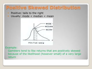
Downloaded 252 times


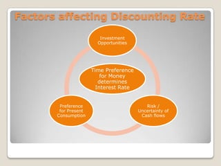

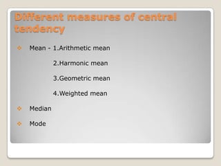
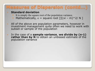
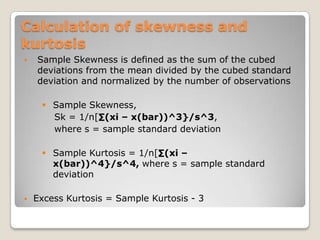
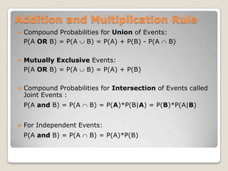
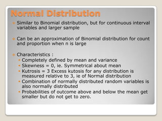
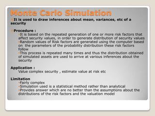
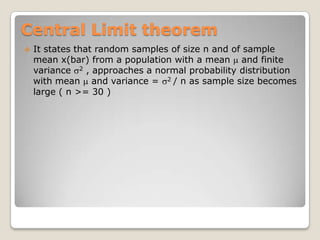
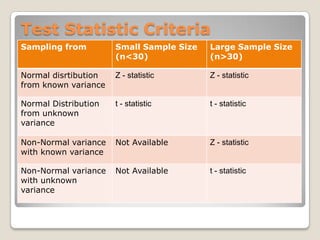
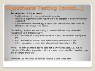
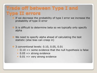
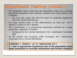
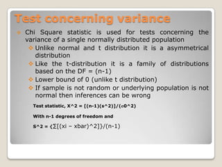
![Dividing the future cash flows by interest rate, we come at present value of future cash flowsFuture Value of Cash FlowsFV3 = (1+i)3PVFV2 = (1+i)2PVPV1230Future Value of cash flow is always greater than present value of cash flowFV1 = (1+i)PVFinding FVs (moving to the right on a time line) is called compounding. Compounding involves earning interest on interest for investments of more than one period.AAAAAAA12345670PV1 = A/(1+r)PV2 = A/(1+r)2PV3 = A/(1+r)3PV4 = A/(1+r)4etc.etc.PerpetuitiesPerpetuity is a series of constant payments, A, each period forever.PVperpetuity = [A/(1+i)t] = A [1/(1+i)t] = A/iIntuition:Present Value of a perpetuity is the amount that must invested today at the interest rate i to yield a payment of A each year without affecting the value of the initial investment.](https://image.slidesharecdn.com/quantitativemethods-110529150506-phpapp01/85/Quantitative-methods-15-320.jpg)
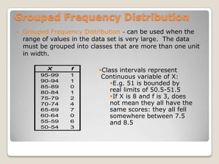
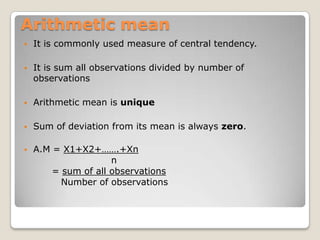


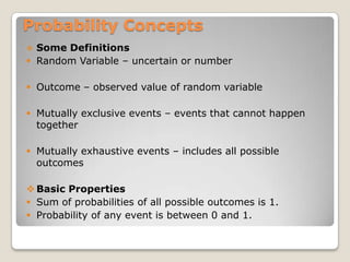
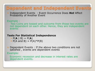
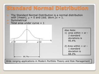
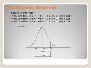
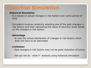
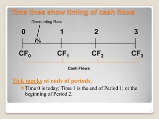
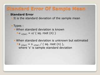
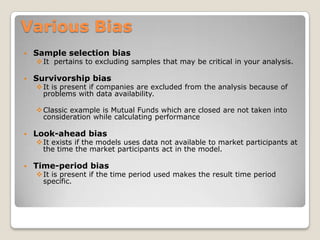
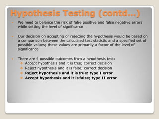
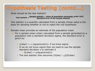
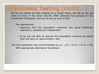
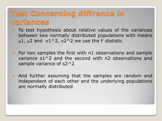
![Mathematically,= square root [∑(xi – m)^2/ N ]](https://image.slidesharecdn.com/quantitativemethods-110529150506-phpapp01/85/Quantitative-methods-84-320.jpg)

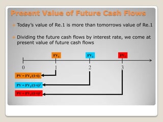
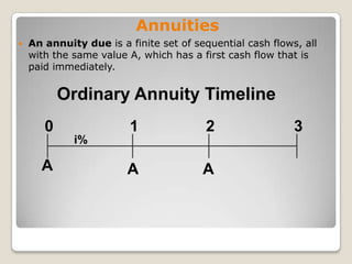
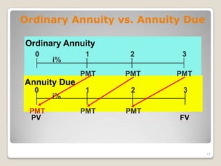
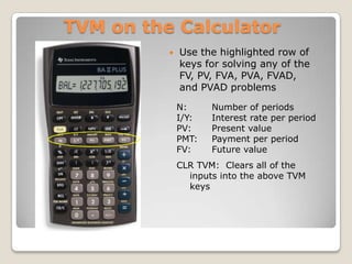
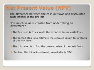
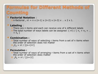
This document provides an overview of quantitative methods topics including time value of money, discounted cash flow applications, probability concepts, and statistical measures. Key points discussed include calculating present and future value of cash flows using timelines and interest rates, as well as methods for analyzing investments like net present value, internal rate of return, and holding period return. Common statistical concepts are also summarized such as measures of central tendency, frequency distributions, and histograms.


