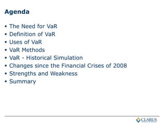
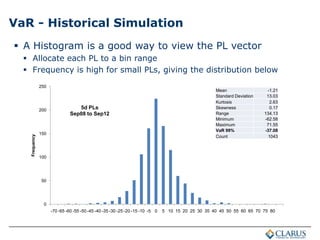
Value at Risk (VaR) is a risk measurement technique used to estimate potential losses that could occur from market risk over a specified time period. The document discusses the need for VaR, how it is defined and calculated using historical simulation, its uses, strengths and weaknesses. It emphasizes that VaR should not be used alone and other risk measures like tail measures and stress testing are also important.

1. Value at Risk
June 7, 2013
Amir Khwaja
www.clarusft.com

2. Agenda
 The Need for VaR
 Definition of VaR
 Uses of VaR
 VaR Methods
 VaR - Historical Simulation
 Changes since the Financial Crises of 2008
 Strengths and Weakness
 Summary

3. The Need for VaR
 Different Asset Classes use their own measures
 Fixed Income – Duration
 Interest Rates – DV01
 FX – Currency position
 Commodity – Number of contracts
 Equities – Number of shares
 Using these to compare risk in these portfolios is like
comparing apples and oranges
 An investor or owner needs a simple measure that can be
used in a consistent way to compare risk between these
portfolios
 And with the ability to aggregate risk appropriately
 Value at Risk is that risk measure

4. Definition of VaR
 How much could we lose over a specified holding period
with a defined probability
 So if a portfolio has a VaR of $20 million
 We need to know the confidence level used to calculate
 We need to know the holding period (time horizon)
 Say confidence level is 99% and holding period is 5 days
 This then means “We would expect to lose $20 million
or more over a 5 day period, in 1 out of 100 business
days”
 Note it does not tell us whether on that 1 day we could
lose $21 million or $200 million!
 So if we are relying only on VaR for the answer to that
then we are going to be in trouble
 For that we need Tail Measures or Stress Testing

5. Uses of VaR
 Made public by JP Morgan in 1994 with RiskMetrics
 Widely adopted in the industry very quickly after that
 Particularly for Derivatives where measures such as gross
notional or position in contracts units, are not that
insightful
 Basel II Capital Accord for Market Risk – 1995
 Internal Model Capital is VaR times a multiplier set for each
bank by its regulator as between 3 & 4
 Banks report VaR in Annual Financial Statements – 1997
 Internal 1d VaR and Regulatory 10d VaR
 Clearing Houses for Initial Margin – 1999 (LCH SwapClear)
 Margin from defaulting member used to cover the market risk
loss for the period it takes to close-out the portfolio

6. VaR Methods
 Three main methods
 Parametric (aka Variance-Covariance or Delta-Gamma)
 Historical Simulation
 Monte-Carlo Simulation
 Different assumptions, calculation steps, compute
efficiency but similar numbers for standard portfolios
 The most common is Historical Simulation
 As easiest to understand
 Simple assumptions on distributions of returns
 So if for our $20 million VaR portfolio, we also said that we
had used 5 Years of history as well as 99% and 5d
 We would say that “given how the market has performed
in the past 5 years” our VaR estimate is $20 million

7. VaR - Historical Simulation
 It relies on choosing
 A historical period, e.g. 4 Years
 A holding period e.g. 5 days
 Generating daily holding period returns in this period
 Calculating the P&L impact on a portfolio by applying
these returns to today
 Ordering the P&L outcomes by decreasing loss
 Interpolating for a chosen confidence level e.g. 99%

8. VaR - Historical Simulation
-80.00
-60.00
-40.00
-20.00
0.00
20.00
40.00
60.00
80.00
USD 5Y Swap Rate
5d returns (bps)
Sep08 to Sep12
20Nov08 > -60bps
13Dec10 > 20bps

9. VaR - Historical Simulation
 Assume our portfolio has a PV01 of $1million
 Assume for simplicity that USD 5Y Swap is the only risk factor
 For a 1 bps rise in the 5Y Swap rate, our Profit will be $1m
 For a 1 bps fall in the 5Y Swap rate, our Loss will be $1m
 We can calculate the PL Series for our portfolio by multiplying the
bps returns on each day by $1 million, which is shown below
-80.00
-60.00
-40.00
-20.00
0.00
20.00
40.00
60.00
80.00
Profit Loss
Sep08 to Sep12
20Nov08 > $60m

10. VaR - Historical Simulation
 This PL Series
 Has a PL value for each business day from 5 Sep 08 to 4 Sep 12
 A total count of 1043 values
 Each corresponds to a specific scenario date, starting on 5 Sep 08
 The first element represents the PL outcome of applying the 5-day
return shift between 1 Sep 08 and 5 Sep 08 to todays market data
and todays portfolio
 We call this the PL vector of the portfolio
 The first few elements of which are shown below
-26.51
-5.97
-12.75
-6.47
-3.29
-15.83
-14.76
-37.08
-9.98
-16.55
22.76
71.55
09/05/2008
09/08/2008
09/09/2008
09/10/2008
09/11/2008
09/12/2008
09/15/2008
09/16/2008
09/17/2008
09/18/2008
09/19/2008
09/22/2008
For these dates

11. VaR - Historical Simulation
 The PL vector can then be re-ordered by decreasing loss
 Keeping a note of the scenario date and PL of each
 The first part of this is shown below
1
2
3
4
5
6
7
8
9
10
11
11/20/2008
12/17/2008
10/21/2008
10/22/2008
11/21/2008
06/17/2009
08/14/2009
12/18/2008
10/06/2008
10/07/2008
09/16/2008
-62.58
-56.16
-47.79
-46.24
-44.95
-42.47
-41.29
-39.73
-39.62
-37.45
-37.08
For these datesRe-order by PL
 Now we can determine the VaR
 Which we will define as 99% or the loss of the 11th worst PL
 (We could define as 10th worst or interpolate between 10th and 11th)
 So VaR is $37.08m
 Occurs on the scenario date of 16-Sep-08, we call this the VaR Date
 This is the week of Lehman’s bankruptcy filing
VaR Date

12. VaR - Historical Simulation
0
50
100
150
200
250
-70 -65 -60 -55 -50 -45 -40 -35 -30 -25 -20 -15 -10 -5 0 5 10 15 20 25 30 35 40 45 50 55 60 65 70 75 80
Frequency
5d PLs
Sep08 to Sep12
Mean -1.21
Standard Deviation 13.03
Kurtosis 2.63
Skewness 0.17
Range 134.13
Minimum -62.58
Maximum 71.55
VaR 99% -37.08
Count 1043
 A Histogram is a good way to view the PL vector
 Allocate each PL to a bin range
 Frequency is high for small PLs, giving the distribution below

13. VaR - Historical Simulation
 Zooming in to the largest losses
Mean -1.21
Standard Deviation 13.03
Kurtosis 2.63
Skewness 0.17
Range 134.13
Minimum -62.58
Maximum 71.55
VaR 99% -37.08
Count 1043
11th largest loss
Largest loss
Expected Shortfall

14. Changes since the Financial Crises of 2008
 Basell Capital Accord, introduced Stressed VaR
 So Trading Book Capital is the higher of Firm’s Multiplier *
VaR or Multiplier * Stressed VaR
 Where Stressed VaR covers a period of Market Stress
 The Financial Crises of 2008 qualifies as a period of stress
for most major markets
 Wider use of Tail measures
 Expected Shortfall (ES) or Worst Case Loss (WCL)
 Renewed focus that Stress testing must be performed and
the definition and results of these discussed within the firm
and with regulators
 Hence US & European Regulatory Stress Tests

15. Strengths and Weaknesses
 Strengths
 Reduces risk to a single $ amount
 Mark to market based measure (not original notional)
 Compare risk of different asset class portfolios
 Aggregate risk across portfolios
 Widely used since 1994
 Weaknesses
 Reduces risk to a single $ amount
 Assumptions may be complex
 Depends on market prices being observable and similar
behaviour to that observed in the past
 Long-tailed properties of financial markets
 Portfolio diversification is not there in a Crisis
 So correlation goes to 1

16. Summary
 It is crucial to understand any assumptions
 For VaR, these are
 Method e.g. Historical Simulation
 Confidence level e.g. 99.7%
 Holding Period e.g. 5 days
 Historical Period Used e.g. 5 Years
 And not use just a single VaR measure
 Or indeed discard VaR (and replace with what?)
 So, in addition to VaR
 Use Tail Measures e.g. ES or WCL
 Stress Tests – Historical and Hypothetical
 Independent price verification
 Gross measures

17. Contact Details
Our LinkedIn Page: Clarus Financial Technology
Our Website: www.clarusft.com
My contact details: amir@clarusft.com