Downloaded 211 times
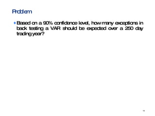
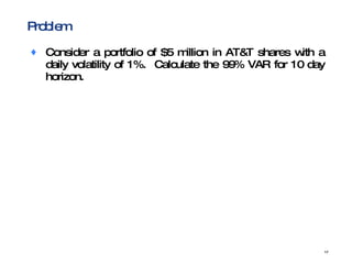
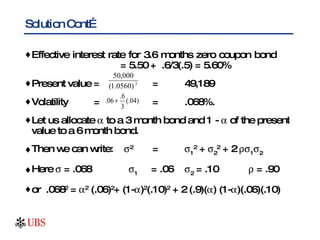
![Solution Cont… Now consider $1,050,000 received after 0.8 years. It can be considered a combination of 6 month and 12 month positions. Interpolating the interest rate we get: = .066 Volatility = [.1 + (3.6/6)(0.1) ] = 0.16 Present value of cash flows = = $997,662](https://image.slidesharecdn.com/valueatrisksep22-100103003529-phpapp02/85/Value-At-Risk-Sep-22-71-320.jpg)
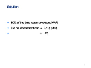
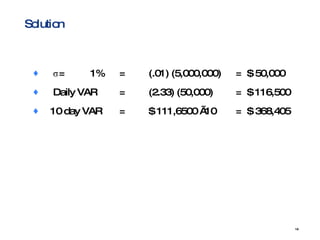
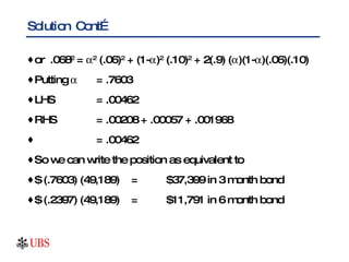
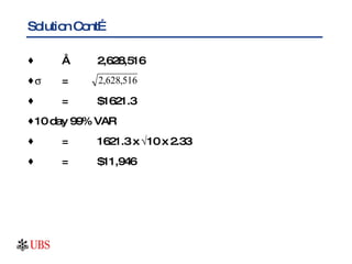
![Solution Cont… Let 1 , 2 , 3 be the volatilities of the 3 month, 6 months, 12 months bonds and 12, 13 , 23 be the respective correlations. Then 2 = 1 2 + 2 2 + 3 2 + 2 12 1 2 + 2 23 2 3 + 2 13 1 3 = [(37,399) 2 (.06) 2 + (331,380) 2 (.10) 2 + (678,074) 2 (.20) 2 + (2) (37,399) (331,380) (.06) (.10) (.90) + (2) (331,380) (678,074) (.10) (.20) (.70) + (2) (37,399) (678,074) (.06) (.20) (.60)] x 10 -4 = [5,035,267 + 1,098,127,044 + 18,391,373,980 + 133,847,431+6,291,604,539+365,173,769]x10 -4](https://image.slidesharecdn.com/valueatrisksep22-100103003529-phpapp02/85/Value-At-Risk-Sep-22-74-320.jpg)

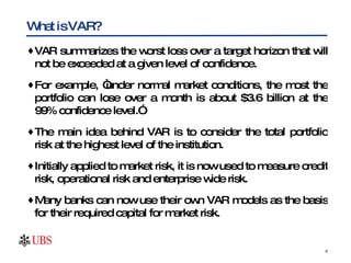
Value at Risk (VAR) summarizes the worst potential loss over a target period at a given confidence level, accounting for risks across an institution. VAR is calculated using statistical techniques to estimate losses that may occur but are unlikely to be exceeded. It is used to measure market, credit, operational and enterprise-wide risk and determine capital requirements to withstand unexpected losses.


