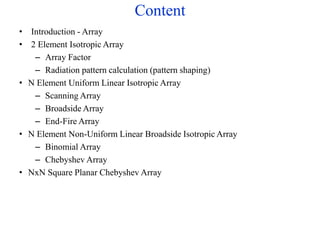
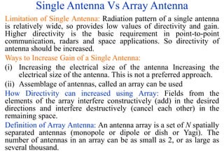
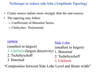
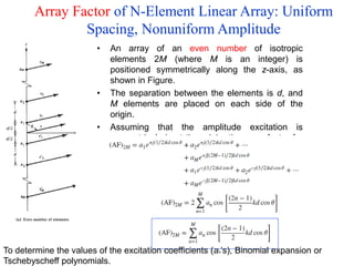
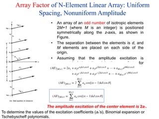
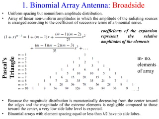
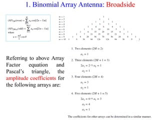
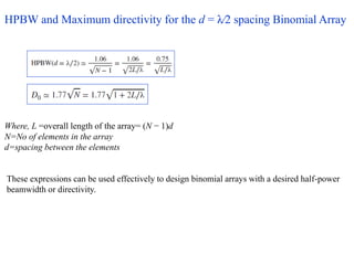
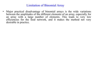
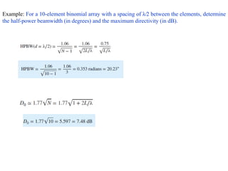
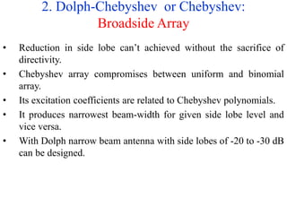
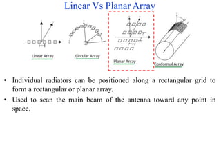
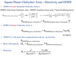
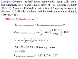
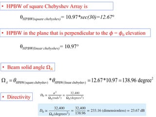
This document discusses different types of antenna arrays, including uniform linear arrays and how their radiation patterns can be shaped. It describes 2-element arrays and calculates their array factors. It also covers N-element uniform linear arrays, including scanning arrays with a progressive phase shift between elements to direct the main beam, broadside arrays with in-phase elements, and end-fire arrays with a phase shift to direct the main beam along the array axis. Non-uniform arrays like binomial and Chebyshev arrays are also introduced. Pattern multiplication is used to calculate approximate radiation patterns from array factors and element patterns.
![Shaping the Pattern of Array
• The total field of the array is determined by the vector
addition of the fields radiated by the individual elements.
• Fields from the elements of the array interfere
constructively (add) in the desired directions and interfere
destructively (cancel each other) in the remaining space
[neglecting coupling]
• Approaches to control the shape of the beam
1. the geometrical configuration of the overall array
2. the relative displacement between the elements
3. the excitation amplitude of the individual elements
4. the excitation phase of the individual elements
5. the relative pattern of the individual elements](https://image.slidesharecdn.com/3antennaarraymodlue41-220419112111/85/3_Antenna-Array-Modlue-4-1-pdf-5-320.jpg)
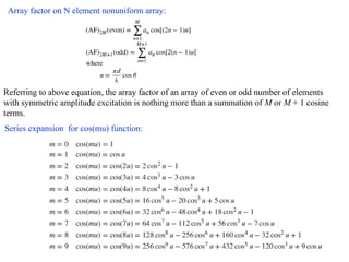
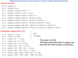
![Pattern Multiplication
Radiation patterns of an array of N identical antennas =
[element pattern Fe (pattern of one of the antennas)] X [the array pattern Fa]
where Fa is the pattern obtained upon replacing all of the actual
antennas with isotropic sources.](https://image.slidesharecdn.com/3antennaarraymodlue41-220419112111/85/3_Antenna-Array-Modlue-4-1-pdf-8-320.jpg)
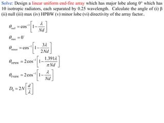
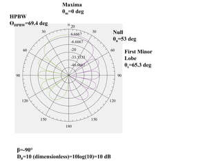
![Solve:
Consider a two Hz dipole element array, where d=λ/4 and the normalized field is given
by
E=cos (𝜃element) cos (1/2[kdcos 𝜃array+β]).
Calculate the approximate pattern using principle of pattern multiplication for the cases
β=0,+90,-90.
To construct the pattern approximately calculate the nulls of the array.](https://image.slidesharecdn.com/3antennaarraymodlue41-220419112111/85/3_Antenna-Array-Modlue-4-1-pdf-9-320.jpg)
![Applying Pattern Multiplication: Array to 2 Hz Dipoles
cos (𝜃element) X cos (𝜋/4cos 𝜃array).
(i) β=0; d=λ/4
E=cos (𝜃element) cos(1/2[kdcos 𝜃array+β]).](https://image.slidesharecdn.com/3antennaarraymodlue41-220419112111/85/3_Antenna-Array-Modlue-4-1-pdf-10-320.jpg)
![cos (𝜃element) X cos (𝜋/4 cos 𝜃array+ 𝜋/4).
(ii) β=+90; d=λ/4
E=cos (𝜃element) cos(1/2[kdcos 𝜃array+β]).](https://image.slidesharecdn.com/3antennaarraymodlue41-220419112111/85/3_Antenna-Array-Modlue-4-1-pdf-11-320.jpg)
![cos (𝜃element) X cos (𝜋/4cos 𝜃array - 𝜋/4).
(iii) β=-90; d=λ/4
E=cos (𝜃element) cos(1/2[kdcos 𝜃array+β])](https://image.slidesharecdn.com/3antennaarraymodlue41-220419112111/85/3_Antenna-Array-Modlue-4-1-pdf-12-320.jpg)
![1
1
max
1
minor
1
HPBW
HPBW max
cos
cos
2
cos
2
3
cos
2 2
2.782
cos
2 2
2 | |
null
h
kd
d Nd
d
d Nd
d Nd
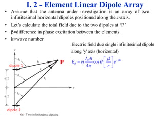
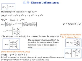
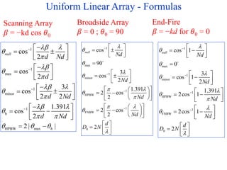
II. N - Element Uniform Array
Case 1. Scanning Array [Array with Maximum Field in an Arbitrary Direction]](https://image.slidesharecdn.com/3antennaarraymodlue41-220419112111/85/3_Antenna-Array-Modlue-4-1-pdf-16-320.jpg)
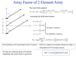
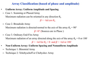
![• If the maximum radiation of an array directed normal to the
axis of the array [broadside; 𝜃0 = 90◦]
• Now let us calculate the condition for broadside radiation.
• First maximum of the array factor occurs when
𝜓 = kd cos 𝜃 + 𝛽 = 0
• Since it is desired to have the first maximum directed toward
𝜃0 = 90, then
𝜓 = kd cos 𝜃 + 𝛽 |𝜃=90◦ = 𝛽 = 0
• Thus to have the maximum of the array factor of a uniform
linear array directed broadside to the axis of the array, it is
necessary that all the elements have the same phase
excitation (in addition to the same amplitude excitation).
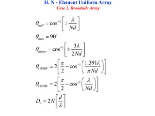
II. N - Element Uniform Array
Case 2. Broadside Array](https://image.slidesharecdn.com/3antennaarraymodlue41-220419112111/85/3_Antenna-Array-Modlue-4-1-pdf-18-320.jpg)
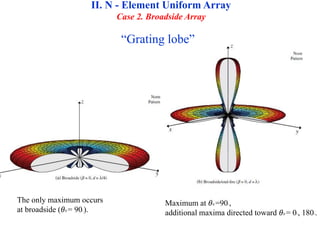
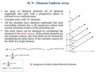
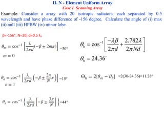
![• If the maximum radiation of an array directed along the axis of the array
[broadside; 𝜃0 = 0 or 180◦]
• Now let us calculate the condition for broadside radiation.
• First maximum of the array factor occurs when
𝜓 = kd cos 𝜃 + 𝛽 = 0
• To direct the first maximum toward 𝜃0 = 0
𝜓 = kd cos 𝜃 + 𝛽|𝜃=0◦ = kd + 𝛽 = 0
𝛽 = −kd
• To direct the first maximum toward 𝜃0 = 180
𝜓 = kd cos 𝜃 + 𝛽|𝜃=180◦ = −kd + 𝛽 = 0
𝛽 = kd
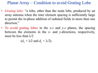
• If the element separation is d = λ∕2, end-fire radiation exists
simultaneously in both directions (𝜃0 = 0 and 𝜃0 = 180).
• To avoid any grating lobes dmax < λ∕2.
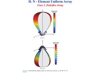
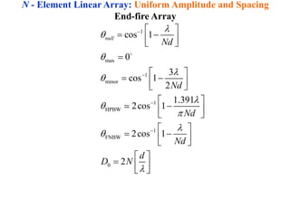
II. N - Element Uniform Array
Case 3. End-fire Array](https://image.slidesharecdn.com/3antennaarraymodlue41-220419112111/85/3_Antenna-Array-Modlue-4-1-pdf-22-320.jpg)
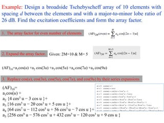
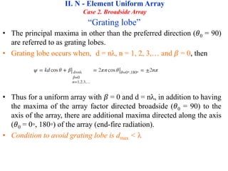
![4. Determine z0 from the ratio of major-to-minor lobe intensity (R0), using
Where,
R0 (dB)=20 log10(R0)
R0 = Major-to-side lobe voltage ratio=10^(26/20)=20.
P is an integer equal to one less than the number of array elements=2M-1=10-1=9.
5. Substitute cosu=z/z0 in the Array factor, calculated in step 3
(AF)10=
a 1 {[z/z0)] }+
a2 {4 [z/z0]3 − 3 [z/z0] }+
a3 {16 [z/z0]5 − 20 [z/z0]3 + 5 [z/z0] }+
a4 { 64 [z/z0]7 − 112 [z/z0]5 + 56 [z/z0]3 − 7 [z/z0] }+
a5 { 256 [z/z0]9 − 576 [z/z0]7 + 432 [z/z0]5 − 120 [z/z0]3 + 9 [z/z0] }
(AF)10=
a1cos(u) +
a2 {4 cos3 u − 3 cos u }+
a3 {16 cos5 u − 20 cos3 u + 5 cos u }+
a4 {64 cos7 u − 112 cos5 u + 56 cos3 u − 7 cos u }+
a5 {256 cos9 u − 576 cos7 u + 432 cos5 u − 120 cos3 u + 9 cos u }
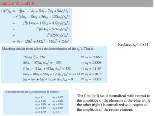
z0=1.0851](https://image.slidesharecdn.com/3antennaarraymodlue41-220419112111/85/3_Antenna-Array-Modlue-4-1-pdf-41-320.jpg)
![6. To determine the excitation coefficients (an’s),
Equate the array factor calculated in Step 5, with Chebyshev polynomial Tm(z)
Where, m=(2M)-1=10-1=9.
….(A)
….(B)
Equate (A) and (B)
(AF)10=
a 1 {[z/z0)] }+
a2 {4 [z/z0]3 − 3 [z/z0] }+
a3 {16 [z/z0]5 − 20 [z/z0]3 + 5 [z/z0] }+
a4 { 64 [z/z0]7 − 112 [z/z0]5 + 56 [z/z0]3 − 7 [z/z0] }+
a5 { 256 [z/z0]9 − 576 [z/z0]7 + 432 [z/z0]5 − 120 [z/z0]3 + 9 [z/z0] }
Tschebyscheff
polynomial of
order 9](https://image.slidesharecdn.com/3antennaarraymodlue41-220419112111/85/3_Antenna-Array-Modlue-4-1-pdf-42-320.jpg)
![3_Antenna Array [Modlue 4] (1).pdf](https://image.slidesharecdn.com/3antennaarraymodlue41-220419112111/85/3_Antenna-Array-Modlue-4-1-pdf-54-320.jpg)


![Getting Started with Apache Spark: Big Data Made Simple [Free Meetup]](https://cdn.slidesharecdn.com/ss_thumbnails/apachesparkgettingstarted-260203175547-8361bcc3-thumbnail.jpg?width=640&height=640&fit=bounds)


