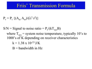
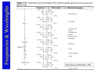
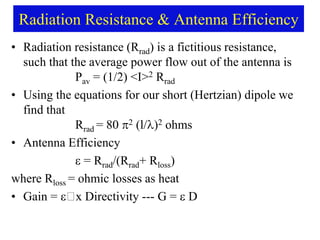
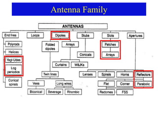
This document provides an overview of antennas and transmission lines. It discusses Maxwell's equations, the electromagnetic spectrum, and how to characterize antennas in terms of directivity, power patterns, gain, effective area, and efficiency. Specific antenna types covered include dipoles, monopoles, Yagi arrays, log-periodic antennas, parabolic reflectors, patches, and arrays. Transmission lines are also briefly introduced.

1. A Brief Introduction to Antennas
& Transmission Lines
Prof. John Vesecky
Outline of Presentation
• Maxwell’s Equations & EM Waves
• EM Spectrum
• Antenna Characterization
• Dipoles and Monopoles
• End Fires (Yagis & Log-Periodics)
• Apertures (Parabolic Reflectors)
• Patches & Arrays
• Transmission Lines
• Friis’ Equation

2. • I. Outline for Wire, Aperture and Patch
Antennas
• EM Spectrum
• Antenna Characterization
• Dipoles and Monopoles
• End Fires (Yagis & Log-Periodics)
• Apertures (Parabolic Reflectors)
• Patches & Arrays

3. EM waves in free space
• v2 = 1/(oµo) so v = 3 x 108 m/s
 o = 8.855 x 10-12 Farads/m
– µo = 1.2566 x 10-6 Henrys/m
• EM waves in free space propagate
freely without attenuation
• What is a plane wave?
– Example is a wave propagating
along the x-direction
– Fields are constant in y and z
directions, but vary with time
and space along the x-direction
– Most propagating radio (EM)
waves can be thought of a plane
waves on the scale of the
receiving antenna

4. E & H fields and
Poynting Vector for Power Flow
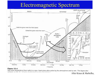
• Power flow in the EM field
– P = E x H (P is Poynting vector)
• In free space E and H are perpendicular
• P is perpendicular to both E and H
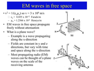
• Plane wave radiated by an antenna
– P = E x H -> Eo Ho Sin2(t-kx)
– P = [Eo
2/] Sin2(t-kx)
– Pavg = (1/2) [Eo
2/] in W/m2
  = impedance of free space
= 377 

5. Electromagnetic Spectrum
After Kraus & Marhefka,

6. Frequencies
&
Wavelengths
After Kraus & Marhefka, 2003

7. RF Bands, Names & Users
After Kraus & Marhefka,
2003

8. Radiation from a Short Antenna Element or Hertzian Dipole
• Using the Electrodynamic
Retarded Potential A (Vector) we
can derive (see Ramo et al., 1965
or Skilling, 1948, Ulaby, 2007 or
any EM theory book)
E and H fields associated with a
small element of current of
length l (<< ) that has the
current varying as
i = I Sin (t)
• This could be a wire or charge
moving in space, e.g. in the
plasma of the ionosphere or a star
or nebula
• E and H fields at r could be in
the r,  or  directions

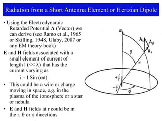
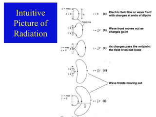
9. Radiation from a Short Antenna Element or Hertzian Dipole
A(r) = (µo/4) (e-jkr/r)∫V [J (e-jkr’/r’)] dv’
H = (1/µo) curl A
• H = (Io l k2/4) e-jkr [j/(kr) + 1/(kr)2] sin 
• Hr = 0 and H = 0
E = (1/jo) curl H
• Er = (2Io l k2/4) o e-jkr [1/(kr)2 - j/(kr)3]
• E = (Io l k2/4) o e-jkr [j/kr + 1/(kr)2 - j/(kr)3]
o = Sqrt(µo/o) = 377 Ω

10. Radiation from a Short Antenna Element
• Terms that fall off as 1/r3 or 1/r2 are small at any
significant distance from an antenna
• Remaining “radiation” terms fall off only as 1/r
and thus transmit energy for long distances also
E and H fields are in phase
• When one is in the “near field” the 1/r3 or 1/r2
the other terms are important

11. Antenna Field Zones
• The dividing line
“Rule of Thumb” is R
= 2L2/
• The near field or
Fresnel zone is r < R
• The far field or
Fraunhofer zone is
r > R

12. Intuitive
Picture of
Radiation

13. Intuitive Picture of Radiation

14. Polarization of EM Waves
AR = Axial Ratio

15. Simple Dipole Antenna

16. Antenna Characterization
• Directivity
• Power Pattern
• Antenna Gain
• Effective Area
• Antenna Efficiency

17. Antenna Directivity
• An omnidirectional antenna radiates power
into all directions (4 steradians) equally
• Typically an antenna wants to beam
radiation in a particular direction
• Directivity
D = 4/,  is the antenna beam
solid angle
• What  would be for one octant
(x,y,z all > 0) ?

18. • Pn(, ) =
S()/S()max
• S()
= Poynting vector
magnitude
= [E
2 + E
2]/
  = 376.7 free
space)
After Kraus (2003)
Normalized Antenna Power Pattern

19. Antenna Gain
• Gain is like directivity, but includes losses as well
• G() ≈ /() is nondimensional° --
 accounts for losses
• dB = 10 log(x/xref) -- always refers to power
• Gain for Typical Antenna with significant
directivity
• G() ≈ 2500/(° °), taking into account
beam shape and typical losses

20. Estimating Effective Antenna Area & Gain
• Definition: G = (4 Ae)/2
• Ae =  A, where A is the physical area
and  is the antenna efficiency
• To get the average power available at the antenna
terminals we use
• Pav,Ant = Pav,Poynting (Average Poynting Flux) Ae
• A crude estimate of G can be obtained by letting
  ≈ (/d), where d is the antenna dimension along the
direction of the angle  -- big antenna means small 
– and G() ≈ /()

21. Radiation Resistance & Antenna Efficiency
• Radiation resistance (Rrad) is a fictitious resistance,
such that the average power flow out of the antenna is
Pav = (1/2) <I>2 Rrad
• Using the equations for our short (Hertzian) dipole we
find that
Rrad = 80 2 (l/)2 ohms
• Antenna Efficiency
 = Rrad/(Rrad+ Rloss)
where Rloss = ohmic losses as heat
• Gain =  x Directivity --- G = D

22. Antenna Family

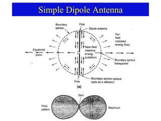
23. Short Dipole Antenna Analysis
• Consider a finite, but short antenna with
l << situated in free space
• Current is charging the uniformly
distributed capacitance of the antenna
wire & so has a maximum at the middle
and tapers toward zero at the ends
• Each element dl radiates per our radiation
equations (previous slide), namely
• In the far field
E = ( I dl sin/(2 r )) cos {[t-(r/c)]}
• The  direction is in the same plane as the
element dl and the radial line from
antenna center to observer and
perpendicular to r

24. Short Dipole Antenna Result
• The resultant field at the observer at r is the sum of the
contributions from the elemental lengths dl
– Each contribution is essentially the same except that the current I varies
– Radiation contribution to the sum is strongest from the center and
weakest at the ends
• This can be summarized as the rms field strength in volts per
meter as
E,rms = [ Io le sin/(2 r )] -- V/m
• What do you think the effective length le & current Io are?
• The radiated power is
Pav = (E,rms)2/(2

25. Modifications for Half Wavelength Dipole
• For antennas comparable in
size to 
– Current distribution is not linear
– Phase difference between
different parts of the antenna
• Current distribution on
/2 dipole
– Antenna acts like open circuit
transmission line with uniformly
distributed capacitance
– Sinusoidal current distribution
results

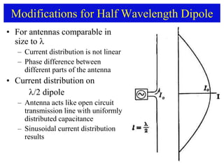
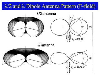
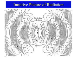
26. Fields from /2 Dipole
• To take account of the phase
differences of the contributions
from all the elements dl we
need to integrate over the
entire length of the antenna as
shown by the figure (from
Skilling, 1948)
E = ∫±/4 ( Io sine/2 re )
cos kx cos [t-(re/c)] dx
– Integral is from -/4 to /4, i.e.
over the antenna length
• Result of integration
E = (Io/2r) cos [t-(r/c)]
{cos [( /2) cos] / sin}
• We know that Er = E= 0 as
for the Hertzian dipole

27. /2 and  Dipole Antenna Pattern (E-field)

28. Monopole over a Conducting Plane -- /4 Vertical

29. /4 Vertical over Ground Plane & Real Earth
• Solid line is for perfectly conducting Earth
• Shaded pattern shows how the pattern is modified by a more
realistic Earth with dielectric constant k = 13 and conductivity G =
0.005 S/m

30. Yagi - Uda
• Driven element induces currents in
parasitic elements
• When a parasitic element is slightly
longer than /2, the element acts
inductively and thus as a reflector -
- current phased to reinforce
radiation in the maximum direction
and cancel in the opposite direction
• The director element is slightly
shorter than/2, the element acts
inductively and thus as a director --
current phased to reinforce
radiation in the maximum direction
and cancel in the opposite direction
• The elements are separated by ≈
0.25

31. 3 Element
Yagi
Antenna
Pattern

32. 2.4 GHz Yagi with 15dBi Gain
• G ≈ 1.66 * N (not dB)
• N = number of
elements
• G ≈ 1.66 *3 = 5
= 7 dB
• G ≈ 1.66 * 16 =
27 = 16 dB

33. • A log periodic is an extension of the Yagi idea to a broad-band,
perhaps 4 x in wavelength, antenna with a gain of ≈ 8 dB
• Log periodics are typically used in the HF to UHF bands
Log-Periodic Antennas

34. Parabolic Reflectors
• A parabolic reflector
operates much the same
way a reflecting
telescope does
• Reflections of rays from
the feed point all
contribute in phase to a
plane wave leaving the
antenna along the
antenna bore sight (axis)
• Typically used at UHF
and higher frequencies

35. Stanford’s Big Dish
• 150 ft diameter dish
on alt-azimuth mount
made from parts of
naval gun turrets
• Gain ≈ 4  A/2
≈ 2 x 105 ≈ 53 dB
for S-band (l ≈15 cm)

36. Patch Antennas
• Radiation is from two “slots” on left and right edges of patch where
slot is region between patch and ground plane
• Length d = /r
1/2 Thickness typically ≈ 0.01 
• The big advantage is conformal, i.e. flat, shape and low weight
• Disadvantages: Low gain, Narrow bandwidth (overcome by fancy
shapes and other heroic efforts), Becomes hard to feed when complex,
e.g. for wide band operation
After Kraus & Marhefka, 2003

37. Patch Antenna Pattern

38. Array Antennas

39. Patch Antenna Array for Space Craft
• The antenna is composed
of two planar arrays, one
for L-band and one for C-
band.
• Each array is composed of
a uniform grid of dual-
polarized microstrip
antenna radiators, with
each polarization port fed
by a separate corporate
feed network.
• The overall size of the
SIR-C antenna is 12.0 x
3.7 meters
• Used for synthetic
aperture radar

40. Very Large Array
http://www.vla.nrao.edu/
Organization:
National Radio
Astronomy
Observatory
Location:Socorro NM
Wavelength:
radio 7 mm and larger
Number & Diameter
27 x 25 m
Angular resolution:
0.05 (7mm) to 700
arcsec

41. Radio Telescope Results
• This is a false-color image of the radio galaxy
3C296, associated with the elliptical galaxy
NGC5532. Blue colors show the distribution
of stars, made from an image from the
Digitized Second Palomar Sky Survey, and
red colors show the radio radiation as imaged
by the VLA, measured at a wavelength of
20cm. Several other galaxies are seen in this
image, but are not directly related to the radio
source. The radio emission is from relativistic
streams of high energy particles generated by
the radio source in the center of the radio
galaxy. Astronomers believe that the jets are
fueled by material accreting onto a super-
massive black hole. The high energy particles
are confined to remarkably well collimated
jets, and are shot into extragalactic space at
speeds approaching the speed of light, where
they eventually balloon into massive radio
lobes. The plumes in 3C296 measure 150 kpc
or 480,000 light years edge-to-edge diameter
(for a Hubble constant of 100 km/s/Mpc).
• Investigator(s):ﾊ J.P. Leahy & R.A. Perley.
Optical/Radio superposition by Alan Bridle

42. Impedance Matching
• SWR = (1 + ||)/ (1 - ||)

43. Friis’ Transmission Formula
Pr = Pt {(Aet Aer)/(2 r2)}
S/N = Signal to noise ratio = Pr/(kTsysB)
where Tsys = system noise temperature, typically 10’s to
1000’s of K depending on receiver characteristics
k = 1.38 x 10-23 J/K
B = bandwidth in Hz

44. References 1
• Balanis, C.A., Antenna Theory, Analysis and Design, 2nd
ed., Wiley (1997)
• Cloude, S., An Introduction to Electromagnetic Wave
Propagation & Antennas, Springer-Verlag, New York
(1995)
• Elmore, W. C. and M. A. Heald, Physics of Waves, Dover,
NY (1969)
• Fusco, V. F., Foundations of Antenna Theory &
Techniques, Pearson Printice-Hall (2005)
• Ishimaru, A., Electromagnetic Wave Propagation,
Radiation and Scattering, Prentice-Hall, Englewood Cliffs
NJ (1991)
• Jones, D. S., Acoustic and Electromagnetic Waves, Oxford
Science Publications, Oxford (1989)

45. References 2
• Kraus, J. D., Antennas, 2nd ed., McGraw-Hill, New York
(1988)
• Kraus, J. D. and R. J. Marhefka, Antennas, 3rd ed.,
McGraw-Hill, New York (2004)
• Kraus, J. D., Electromagnetics, 3rd ed., McGraw-Hill, New
York (1983)
• Ramo, S., J. R. Whinnery and T. Van Duzer, Fields and
Waves in Communication Electronics, Wiley NY (1965)
• Skilling, H. H., Fundamentals of Electric Waves, 2nd ed.,
Wiley, NY (1948)
• Ulaby, F., Fundamentals of Applied Electromagnetics, 5th
Ed., Pearson Printice-Hall (2007)